Given numeric data points, find an equation that approximates the data
with a least square fit. This is one of many techniques for getting
an analytical approximation to numeric data.
The problem is stated as follows :
Given measured data for values of Y based on values of X1,X2 and X3. e.g.
Y_actual X1 X2 X3 observation, i
-------- ----- ----- -----
32.5 1.0 2.5 3.7 1
7.2 2.0 2.5 3.6 2
6.9 3.0 2.7 3.5 3
22.4 2.2 2.1 3.1 4
10.4 1.5 2.0 2.6 5
11.3 1.6 2.0 3.1 6
Find a, b and c such that Y_approximate = a * X1 + b * X2 + c * X3
and such that the sum of (Y_actual - Y_approximate) squared is minimized.
(We are minimizing RMS error.)
The method for determining the coefficients a, b and c follows directly
form the problem definition and mathematical analysis given below.
Set up and solve the system of linear equations:
(Each SUM is for i=1 thru 6 per table above, note symmetry)
| SUM(X1*X1) SUM(X1*X2) SUM(X1*X3) | | a | | SUM(X1*Y) |
| SUM(X2*X1) SUM(X2*X2) SUM(X2*X3) | x | b | = | SUM(X2*Y) |
| SUM(X3*X1) SUM(X3*X2) SUM(X3*X3) | | c | | SUM(X3*Y) |
Easy to program, not good data:
lsfit_lect.c
lsfit_lect_c.out
lsfit_lect.java
lsfit_lect_java.out
lsfit_lect.py
lsfit_lect_py.out
lsfit_lect.f90
lsfit_lect_f90.out
lsfit_lect.m similar to c
lsfit_lect_m.out
test_lsfit.py3 Python3 two methods
test_lsfit_py3.out output
test_lsfit2.py3 Python3 two methods
test_lsfit2_py3.out output better
Now, suppose you wanted a constant term to make the fit:
Y_approximate = Y0 + a * X1 + b * X2 + c * X3
Then the linear equations would be:
| SUM( 1* 1) SUM( 1*X1) SUM( 1*X2) SUM( 1*X3) | | Y0 | | SUM( 1*Y) |
| SUM(X1* 1) SUM(X1*X1) SUM(X1*X2) SUM(X1*X3) | | a | | SUM(X1*Y) |
| SUM(X2* 1) SUM(X2*X1) SUM(X2*X2) SUM(X2*X3) | x | b | = | SUM(X2*Y) |
| SUM(X3* 1) SUM(X3*X1) SUM(X3*X2) SUM(X3*X3) | | c | | SUM(X3*Y) |
Note the symmetry! Easy to program.
Note the simultaneous equations, from Lecture 3: |A| x |X| = |Y|
|A| and |Y| easily computable, solve for |X| to get Y0, a, b and c
We now have a simple equation to compute Y approximately from a reasonable
range of X1, X2, and X3.
Y is called the dependent variable and X1 .. Xn the independent variables.
The procedures below implement a few special cases and the general case.
The number of independent variables can vary, e.g. 2D, 3D, etc. .
The approximation equation may use powers of the independent variables
The user may create additional independent variables e.g. X2 = SIN(X1)
with the restriction that the independent variables are linearly
independent. e.g. Xi not equal p Xj + q for all i,j,p,q
Mathematical derivation
The mathematical derivation of the least square fit is as follows :
Given data for the independent variable Y in terms of the dependent
variables S,T,U and V consider that there exists a function F
such that Y = F(S,T,U,V)
The problem is to find coefficients a,b,c and d such that
Y_approximate = a * S + b * T + c * U + d * V
and such that the sum of ( Y - Y_approximate ) squared is minimized.
Note: a, b, c, d are scalars. S, T, U, V, Y, Y_approximate are vectors.
To find the minimum of SUM((Y - Y_approximate)^2)
the derivatives must be taken with respect to a,b,c and d and
all must equal zero simultaneously. The steps follow :
SUM((Y - Y_approximate)^2) = SUM((Y - a*S - b*T - c*U - d*V)^2)
d/da = -2 * S * SUM( Y - a*S - b*T - c*U - d*V )
d/db = -2 * T * SUM( Y - a*S - b*T - c*U - d*V )
d/dc = -2 * U * SUM( Y - a*S - b*T - c*U - d*V )
d/dd = -2 * V * SUM( Y - a*S - b*T - c*U - d*V )
Setting each of the above equal to zero (derivative minimum at zero)
and putting constant term on left, the -2 is factored out,
the independent variable is moved inside the summation
SUM( a*S*S + b*S*T + c*S*U + d*S*V = S*Y )
SUM( a*T*S + b*T*T + c*T*U + d*T*V = T*Y )
SUM( a*U*S + b*U*T + c*U*U + d*U*V = U*Y )
SUM( a*V*S + b*V*T + c*V*U + d*V*V = V*Y )
Distributing the SUM inside yields
a * SUM(S*S) + b * SUM(S*T) + c * SUM(S*U) + d * SUM(S*V) = SUM(S*Y)
a * SUM(T*S) + b * SUM(T*T) + c * SUM(T*U) + d * SUM(T*V) = SUM(T*Y)
a * SUM(U*S) + b * SUM(U*T) + c * SUM(U*U) + d * SUM(U*V) = SUM(U*Y)
a * SUM(V*S) + b * SUM(V*T) + c * SUM(V*U) + d * SUM(V*V) = SUM(V*Y)
To find the coefficients a,b,c and d solve the linear system of equations
| SUM(S*S) SUM(S*T) SUM(S*U) SUM(S*V) | | a | | SUM(S*Y) |
| SUM(T*S) SUM(T*T) SUM(T*U) SUM(T*V) | x | b | = | SUM(T*Y) |
| SUM(U*S) SUM(U*T) SUM(U*U) SUM(U*V) | | c | | SUM(U*Y) |
| SUM(V*S) SUM(V*T) SUM(V*U) SUM(V*V) | | d | | SUM(V*Y) |
Some observations :
S,T,U and V must be linearly independent.
There must be more data sets (Y, S, T, U, V) than variables.
The analysis did not depend on the number of independent variables
A polynomial fit results from the substitutions S=1, T=x, U=x^2, V=x^3
The general case for any order polynomial of any number of variables
may be used with a substitution, for example, S=1, T=x, U=y, V=x^2,
W=x*y, X= y^2, etc to terms such as exp(x), log(x), sin(x), cos(x).
Any number of terms may be used. The "1" is for the constant term.
Using the S,T,U,V notation above, fitting Y_approx to find a, b, c, d
Y_approx = a*S + b*T + c*U + d*V + ...
Choose S = 1.0 thus a is the constant term
Choose T = log(x) thus b is the coefficient of log(x)
Choose U = log(x*x) thus c is the coefficient of log(x*x)
Choose V = sin(x) thus d is the coefficient of sin(x)
see 4 additional terms in lsfit_log.c
Thus our x data, n = 21 samples in code, is fit to
Y_approx = a + b*log(x) + c*log(x*x) + d*sin(x) + ...
By putting the terms in a vector, simple indexing builds the matrix:
A[i][j] = A[i][j] + term_i * term_j summing over n terms using k
lsfit_log.c fitting log and other terms
lsfit_log_c.out
fitting a simple polynomial, 1D
Now, suppose you wanted to fit a simple polynomial:
Given the value of Y for at least four values of X,
Y_approximate = C0 + C1 * X + C2 * X^2 + C3 * X^3
Then the linear equations would be A*X=Y:
| SUM(1 *1) SUM(1 *X) SUM(1 *X^2) SUM(1 *X^3) | | C0 | | SUM(1 *Y) |
| SUM(X *1) SUM(X *X) SUM(X *X^2) SUM(X *X^3) | | C1 | | SUM(X *Y) |
| SUM(X^2*1) SUM(X^2*X) SUM(X^2*X^2) SUM(X^2*X^3) |x| C2 | = | SUM(X^2*Y) |
| SUM(X^3*1) SUM(X^3*X) SUM(X^3*X^2) SUM(X^3*X^3) | | C3 | | SUM(X^3*Y) |
Note that the (i,j) subscript in the A matrix has SUM(X^(i)*X^(j))
for i=0..3, j=0..3
In C, to build A matrix and Y vector for solving simultaneous equations:
// sample polynomial least square fit, nth power, m values of xd and yd
for(i=0; i<n+1; i++)
{
for(j=0; j<n+1; j++)
{
A[i][j] = 0.0;
}
Y[i] = 0.0;
}
for(k=0; k<m; k++)
{
y = yd[k];
x = xd[k];
pwr[0] = 1.0;
for(i=1; i<=n+1; i++) pwr[i] = pwr[i-1]*x;
for(i=0; i<n+1; i++)
{
for(j=0; j<n+1; j++)
{
A[i][j] = A[i][j] + pwr[i]*pwr[j]; // SUM
}
Y[i] = Y[i] + y*pwr[i];
}
}
Solve the simultaneous equations A*X=Y for X[0]=C0, X[1]=C1, X[2]=C2, X[3]=C3
Note that the sum is taken over all observations and the "1" is
just shown to emphasize the symmetry.
Sample code in various languages:
least_square_fit.c really old
least_square_fit_c.out
least_square.py3
least_square_py3.out
test_lsfit.py3 Python3 two methods
test_lsfit_py3.out output
lsfit.py3 just 1D version for copying
peval.py3 just 1D version for copying
least_square_fit.f90
least_square_fit_f90.out
Least_square.rb Ruby class new
test_least_square.rb test
test_least_square_rb.out test output
least_square_fit.java
least_square_fit_java.out
least_square_fit_3d.java
least_square_fit_3d_java.out
least_square_fit_4d.java
least_square_fit_4d_java.out
A specialized version for use later with PDE's
lsfit.java
test_lsfit.java
test_lsfit_java.out
test_lsfit2.java
test_lsfit2_java.out
test_lsfit3.java
test_lsfit3_java.out
test_lsfit4.java
test_lsfit4_java.out
test_lsfit5.java
test_lsfit5_java.out
test_lsfit6.java
test_lsfit6_java.out
test_lsfit7.java
test_lsfit7_java.out
uses simeq.java
The Makefile entry that makes test_lsfit_java.out
test_lsfit_java.out: test_lsfit.java lsfit.java simeq.java
javac -cp . simeq.java
javac -cp . lsfit.java
javac -cp . test_lsfit.java
java -cp . test_lsfit > test_lsfit_java.out
rm -f *.class
least_square_fit.adb
least_square_fit_ada.out
least_square_fit_2d.adb
least_square_fit_2d_ada.out
least_square_fit_3d.adb
least_square_fit_3d_ada.out
least_square_fit_4d.adb
least_square_fit_4d_ada.out
real_arrays.ads
real_arrays.adb
lsfit.ads has 1D through 6D
lsfit.adb
test_lsfit6.adb
test_lsfit6_ada.out
array4d.ads
test_lsfit5.adb
test_lsfit5_ada.out
array5d.ads
test_lsfit4.adb
test_lsfit4_ada.out
array4d.ads
test_lsfit3.adb
test_lsfit3_ada.out
array3d.ads
test_lsfit2.adb
test_lsfit2_ada.out
integer_arrays.ads
integer_arrays.adb
real_arrays.ads
real_arrays.adb
The Makefile entry to make test_lsfit6_ada.out
test_lsfit6_ada.out: test_lsfit6.adb lsfit.ads lsfit.adb \
array3d.ads array4d.ads array5d.ads array6d.ads \
real_arrays.ads real_arrays.adb \
integer_arrays.ads integer_arrays.adb
gnatmake test_lsfit6.adb
./test_lsfit6 > test_lsfit6_ada.out
rm -f test_lsfit
rm -f *.ali
rm -f *.o
similarly for test_lsfit2_ada.out, test_lsfit3_ada.out,
test_lsfit4_ada.out, test_lsfit5_ada.out
Similar code in plain C (up to 7th power in up to 6 or 4 dimensions)
lsfit.h
lsfit.c
test_lsfit.c
test_lsfit_c.out
test_lsfit7.c
test_lsfit7_c.out
test_write_lsfit7.c
test_write_lsfit7_c.out
test_write_lsfit71.c generated
test_write_lsfit72.c generated
Simple one variable versions polyfit polyval
polyfit.h
polyfit.c
polyval.h
polyval.c
test_polyfit.c
test_polyfit_c.out
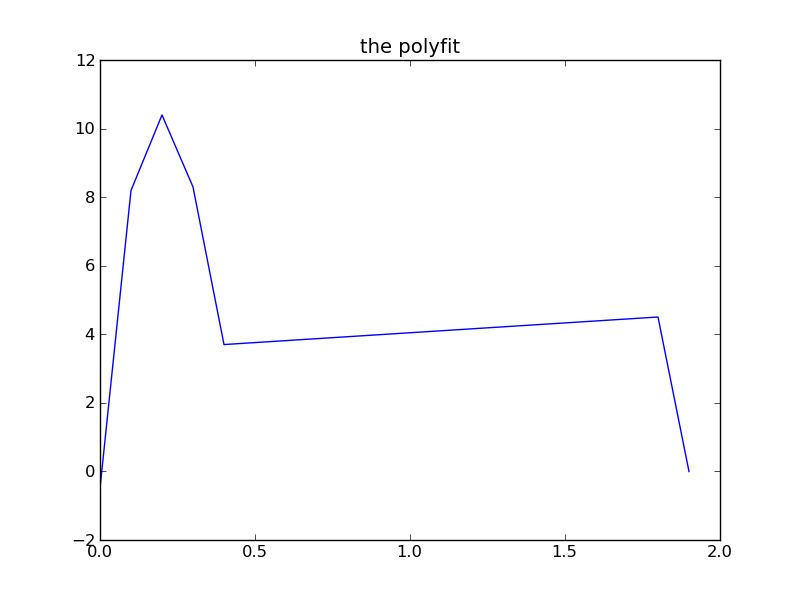
test_polyfit.py3
test_polyfit_py3.out
test_polyfit_py3.png
poly.java
test_poly.java
test_poly_java.out
Poly.scala
Test_poly.scala
Test_poly_scala.out
truncated series vs lsfit for sin(x+y) and sin(x+y+z)
using code from above, another test case:
fit_sin.adb demonstrates that a lsfit to a specified power,
does not give the same coefficients as a truncated approximation,
to the same power, and is a more accurate fit.
fit_sin.adb
fit_sin_ada.out
comparison to very small Matlab code
generic_real_least_square_fit.ada
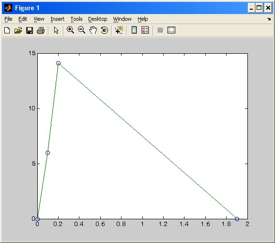
lsfit.m MatLab source code (tiny!)
lsfit_m.out MatLab output and plot
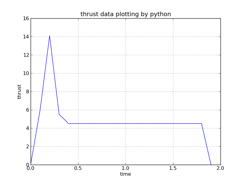
comparison to small Python code
test_polyfit.py Python source code
test_polyfit_py.out Python output and plot


Terms for fitting two and three variables, 2D and 3D
And to see how polynomials in two and three variables may be fit:
Given a value of Y for each value of X, get polynomial with X^2
Y_approximate = C0 + C1 * X + C2 * X^2
Then the linear equations would be:
| SUM(1 *1) SUM(1 *X) SUM(1 *X^2) | | C0 | | SUM(1 *Y) |
| SUM(X *1) SUM(X *X) SUM(X *X^2) | | C1 | | SUM(X *Y) |
| SUM(X^2*1) SUM(X^2*X) SUM(X^2*X^2) |x| C2 | = | SUM(X^2*Y) |
Given a value of Y for each value of X, get polynomial with X^3
Y_approximate = C0 + C1 * X + C2 * X^2 + C3 * X^3
Then the linear equations would be:
| SUM(1 *1) SUM(1 *X) SUM(1 *X^2) SUM(1 *X^3) | | C0 | | SUM(1 *Y) |
| SUM(X *1) SUM(X *X) SUM(X *X^2) SUM(X *X^3) | | C1 | | SUM(X *Y) |
| SUM(X^2*1) SUM(X^2*X) SUM(X^2*X^2) SUM(X^2*X^3) |x| C2 | = | SUM(X^2*Y) |
| SUM(X^3*1) SUM(X^3*X) SUM(X^3*X^2) SUM(X^3*X^3) | | C3 | | SUM(X^3*Y) |
Note that index [i][j] of the matrix has SUM(X^i*X^j)) when subscripts 0..3
Note that the terms for two and three variables in a polynomial are:
two three can optimize
a^0 b^0 a^0 b^0 c^0 constant, "1"
a^1 b^0 a^1 b^0 c^0 just a
a^0 b^1 a^0 b^1 c^0 just b
a^0 b^0 c^1
a^2 b^0 a^2 b^0 c^0 just a^2
a^1 b^1 a^1 b^1 c^0 a*b
a^0 b^2 a^1 b^0 c^1
a^0 b^2 c^0
a^0 b^1 c^1
a^0 b^0 c^2
Then terms with a sum of the powers equal to 3, 4, 5, 6 are available
Note that the matrix has the first row as the sum of each term
multiplied by the first term. The second row is the sum of each
term multiplied by the second term, etc.
The data for the terms is from the raw data sets of
y_actual a b or y_actual a b c
being used to determine a fit
y_approx=F(a,b) or y_approx=F(a,b,c)
Terms for the data point y1 a1 b1 are:
1 a1 b1 a1^2 a1*b1 b1^2 the constant term y1
These terms are multiplied by the first term, "1" and added to row 1.
These terms are multiplied by the second term, "a1" and added to row 2, etc.
Then the terms for data point y2 a2 b2 are:
1 a2 b2 a2^2 a2*b2 b2^2 the constant term y2
These terms are multiplied by the first term, "1" and added to row 1.
These terms are multiplied by the second term, "a2" and added to row 2, etc.
Then the simultaneous equations are solved for the coefficients C1, C2, ...
to get the approximating function
y_approx = F(a,b) = C1 + C2*a + C3*b + C4*a^2 + C5*a*b + C6*b^2
The following sample programs compute the least square fit of
internally generated data for low polynomial powers and compute
the accuracy of the fit in terms of root-mean-square error,
average error and maximum error. Note that the fit becomes exact
when the data is from a low order polynomial and the fit uses at
least that order polynomial.
least_square_fit_2d.c
least_square_fit_2d.out
least_square_fit_3d.c
least_square_fit_3d.out
least_square_fit_4d.c
least_square_fit_4d.out
least_square_fit2d.adb
least_square_fit2d_ada.out
real_arrays.ads
real_arrays.adb
Development of Python 2d and 3d least square fit
polyfit2.py3
polyfit2_py3.out
polyfit3.py3
polyfit3_py3.out
You can translate the above to your favorite language.
Now, if everything works, a live interactive demonstration of
least square fit.
The files needed are:
Matrix.java
LeastSquareFit.java
LeastSquareFitFrame.java
LeastSquareFit.out
LeastSquareFitAbout.txt
LeastSquareFitHelp.txt
LeastSquareFitEvaluate.txt
LeastSquareFitAlgorithm.txt
LeastSquareFitIntegrate.txt
The default parameter is an n, all, point fit.
Then set parameter to 3, for n=3, third order polynomial fit.
Then set parameter to 4 and 5 to see improvement.
Homework 2
Spline fit, possible demonstration
There are many other ways to fit a set of points.
The Spline fit smooths the fit by controlling derivatives.
SplineFrame.java
(Replace "LeastSquareFit" with "Spline" then get same files as above.)
Demonstration to see a different type of fit.
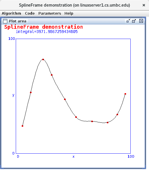 Right click on points, left to right increasing X.
Left click to see plot.
Optional lecture on taylor fit to implement math functions
that may not be availabke in programming language you are using.
optional lecture 4.5
updated 10/30/2021
Right click on points, left to right increasing X.
Left click to see plot.
Optional lecture on taylor fit to implement math functions
that may not be availabke in programming language you are using.
optional lecture 4.5
updated 10/30/2021