<- previous index next ->
A brief introduction to the "Finite Element Method" FEM,
using triangles or tetrahedrons rather than a uniform grid.
The previous Galerkin Method galerkin.pdf
applies with some changes.
There are entire books on FEM and this just covers one small view.
Examples are shown below. The examples are for Degree 1 (linear),
with Order 1 through 4,
Dimension 2 (triangle) and Dimension 3 (tetrahedron)
Some specialty stuff that may be used later:
affine_map_tri.txt triangle mapping
test_affine_map.c test program
test_affine_map.out output
test_affine_map2.c test program
test_affine_map2.out output
test_affine_map.html Maple solution
test_affine_map.mw Maple worksheet
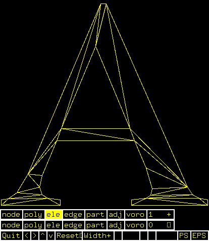
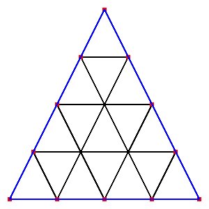
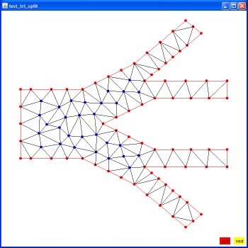
Given a set of coordinates and a boundary path, generate a set of
triangles that cover the interior. Four sets are shown below:
The programs are triangle.c and showme.c run using commands:
triangle A.poly generates file A.1.poly A.1.node A.1.ele
showme -p A.1.poly plots boundary, click on ele to plot triangles
 A.poly initial input (simpler ones follow)
A.1.poly generated by program triangle
A.1.ele generated by program triangle
A.1.node generated by program triangle
triangle -D -a0.01 -q30 -p B.poly generates B.1.*
showme -p B.1.poly wait for menus at bottom, click on ele
A.poly initial input (simpler ones follow)
A.1.poly generated by program triangle
A.1.ele generated by program triangle
A.1.node generated by program triangle
triangle -D -a0.01 -q30 -p B.poly generates B.1.*
showme -p B.1.poly wait for menus at bottom, click on ele
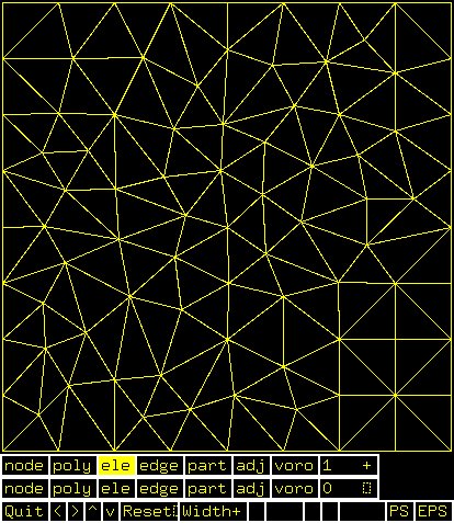 B.poly initial input (square)
B.1.poly generated by program triangle
B.1.ele generated by program triangle
B.1.node generated by program triangle
triangle -D -a0.1 -q30 -p C.poly generates C.1.*
showme -p C.1.poly wait for menus at bottom, click on ele
B.poly initial input (square)
B.1.poly generated by program triangle
B.1.ele generated by program triangle
B.1.node generated by program triangle
triangle -D -a0.1 -q30 -p C.poly generates C.1.*
showme -p C.1.poly wait for menus at bottom, click on ele
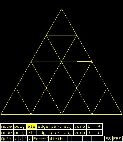 C.poly initial input (triangle)
C.1.poly generated by program triangle
C.1.ele generated by program triangle
C.1.node generated by program triangle
triangle -D -a2.0 -q45 -p D.poly generates D.1.*
showme -p D.1.poly wait for menus at bottom, click on ele
C.poly initial input (triangle)
C.1.poly generated by program triangle
C.1.ele generated by program triangle
C.1.node generated by program triangle
triangle -D -a2.0 -q45 -p D.poly generates D.1.*
showme -p D.1.poly wait for menus at bottom, click on ele
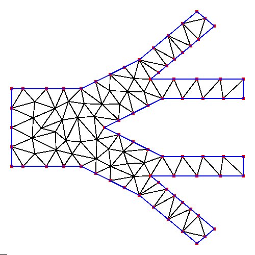
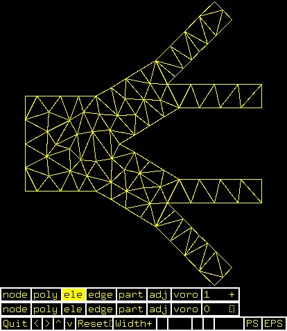 D.poly initial input (channels)
D.1.poly generated by program triangle
D.1.ele generated by program triangle
D.1.node generated by program triangle
triangle.c source code
triangle.help documentation
triangle.readme sample commands
triangle.README README
showme.c source code
note: the C.1.node C.1.ele C.1.poly can be used for fem_check below
C.coord C.tri C.bound by deleting sequence numbers
and extra trailing stuff
D.poly initial input (channels)
D.1.poly generated by program triangle
D.1.ele generated by program triangle
D.1.node generated by program triangle
triangle.c source code
triangle.help documentation
triangle.readme sample commands
triangle.README README
showme.c source code
note: the C.1.node C.1.ele C.1.poly can be used for fem_check below
C.coord C.tri C.bound by deleting sequence numbers
and extra trailing stuff
 C.coord from C.1.node
C.tri from C.1.ele
C.bound from C.1.poly
plot_fem_tri.c plots .coord,.tri,.bound
C.coord from C.1.node
C.tri from C.1.ele
C.bound from C.1.poly
plot_fem_tri.c plots .coord,.tri,.bound
 D.coord from D.1.node
D.tri from D.1.ele
D.bound from D.1.poly
The most basic geometry and several triangle splits:
D.coord from D.1.node
D.tri from D.1.ele
D.bound from D.1.poly
The most basic geometry and several triangle splits:
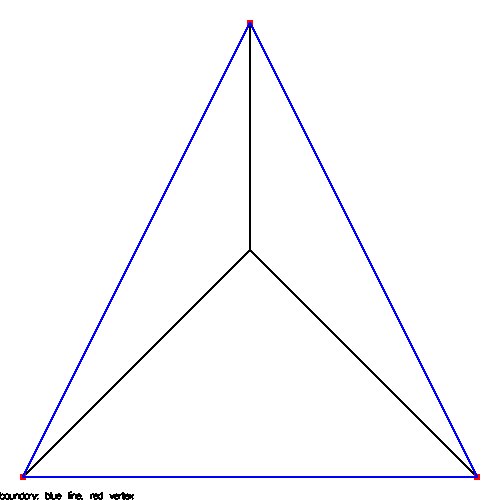 22_t.coord 3 triangles, 4 vertices
22_t.tri 3 boundary, 1 free
22_t.bound
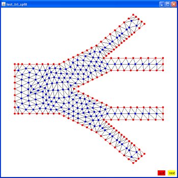
Any FEM group can be split, every triangle becomes 4 triangles that
are one fourth the area and congruent to the original triangles.
This cuts "h" the longest edge in half and should improve accuracy,
up to some limit, at the cost of longer execution time.
do_tri_split.c
22_t.coord 3 triangles, 4 vertices
22_t.tri 3 boundary, 1 free
22_t.bound
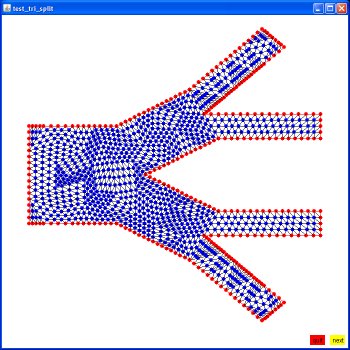
Any FEM group can be split, every triangle becomes 4 triangles that
are one fourth the area and congruent to the original triangles.
This cuts "h" the longest edge in half and should improve accuracy,
up to some limit, at the cost of longer execution time.
do_tri_split.c
 22_ts.coord 12 triangles, 10 vertices
22_ts.tri 6 boundary, 4 free
22_ts.bound
22_ts.coord 12 triangles, 10 vertices
22_ts.tri 6 boundary, 4 free
22_ts.bound
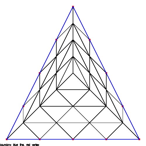 22_tss.coord 48 triangles, 31 vertices
22_tss.tri 12 boundary, 19 free
22_tss.bound
The D.poly from above as original, split once, split again
22_tss.coord 48 triangles, 31 vertices
22_tss.tri 12 boundary, 19 free
22_tss.bound
The D.poly from above as original, split once, split again
 Circles can be split into triangles:
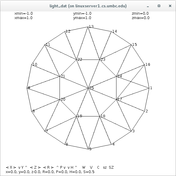 circle_tri.coord
circle_tri.tri
circle_tri.bound
circle_tri.dat
Circles can be grided:
circle_tri.coord
circle_tri.tri
circle_tri.bound
circle_tri.dat
Circles can be grided:
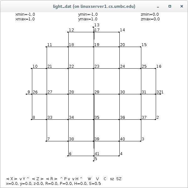 circle_grid.dat
circle_grid.java
Program files that produces the images above:
tri_input.java
tri_split.java
test_tri_split.java
circle_tri.java
The first example of FEM on triangles is a first order in two dimensions.
fem_check21_tri.c source code
fem_check21_tri.out output 22_tri
fem_check21_tria.out output 22_t
fem_check21_tri_C.out output C
additional files needed for execution of the above:
phi_tri.h source code
phi_tri.c source code
phi_tri_cm.h source code
phi_tri_cm.c source code
phi_tri_pts.h source code
phi_tri_pts.c source code
A similar example in Java of FEM on triangles is a first order in two dimensions.
This is an improved version from fem_check21
fem_check21a_tri.java source code
fem_check21a_tri22_t.out output
fem_check21a_tri22_ts.out output
fem_check21a_tri22_tss.out output
additional files needed for execution of the above:
triquad.java source code
simeq.java source code
the test for accuracy of triquad.java are:
test_triquad.java source code
test_triquad.out results, see last two sets
the test for accuracy of triquad_int.c are:
triquad_int.c source code
test_triquad_int.c test code
In order to understand the complexity of the code,
the following figures show one vertex, V1, that is a
part of three triangles, T1, T2 and T3.
For vertex V1 there are three test functions, phi1, phi2 and phi3,
represented by blue for the phi1, yellow for phi2 and red for phi3.
These test functions are shown as linear "hat" functions, yet could
be higher order test functions.
circle_grid.dat
circle_grid.java
Program files that produces the images above:
tri_input.java
tri_split.java
test_tri_split.java
circle_tri.java
The first example of FEM on triangles is a first order in two dimensions.
fem_check21_tri.c source code
fem_check21_tri.out output 22_tri
fem_check21_tria.out output 22_t
fem_check21_tri_C.out output C
additional files needed for execution of the above:
phi_tri.h source code
phi_tri.c source code
phi_tri_cm.h source code
phi_tri_cm.c source code
phi_tri_pts.h source code
phi_tri_pts.c source code
A similar example in Java of FEM on triangles is a first order in two dimensions.
This is an improved version from fem_check21
fem_check21a_tri.java source code
fem_check21a_tri22_t.out output
fem_check21a_tri22_ts.out output
fem_check21a_tri22_tss.out output
additional files needed for execution of the above:
triquad.java source code
simeq.java source code
the test for accuracy of triquad.java are:
test_triquad.java source code
test_triquad.out results, see last two sets
the test for accuracy of triquad_int.c are:
triquad_int.c source code
test_triquad_int.c test code
In order to understand the complexity of the code,
the following figures show one vertex, V1, that is a
part of three triangles, T1, T2 and T3.
For vertex V1 there are three test functions, phi1, phi2 and phi3,
represented by blue for the phi1, yellow for phi2 and red for phi3.
These test functions are shown as linear "hat" functions, yet could
be higher order test functions.
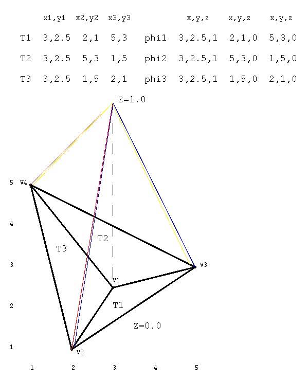 The triangles are in the plane Z=0.0.
All three test functions are at Z=1.0 above the vertex of interest,
V1. All three test functions are at Z=0.0 for all other vertices
in the triangles that include vertex V1.
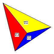
Looking down on the triangles, the three test functions can be seen
to cover the area of the three triangles T1, T2 and T3 with functions
phi1, phi2 and phi3.
The triangles are in the plane Z=0.0.
All three test functions are at Z=1.0 above the vertex of interest,
V1. All three test functions are at Z=0.0 for all other vertices
in the triangles that include vertex V1.
Looking down on the triangles, the three test functions can be seen
to cover the area of the three triangles T1, T2 and T3 with functions
phi1, phi2 and phi3.
 The equation
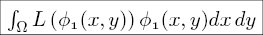 is, in the general case, computed by numerical quadrature
of the linear operator, L, with the dependent variable and
its derivatives replaced by a test function and corresponding
derivatives of the test function.
For the triangulation shown above and for the first equation,
for vertex V1, there are three numerical quadratures that
are summed to get the integral as shown.
The first region, omega is T1 and the test function is phi1.
The second region, omega is T2 and the test function is phi2.
The third region, omega is T3 and the test function is phi3.
In the integral equation, the omega is the sum of T1, T2 and T3.
In the integral equation, the symbol φ1 is phi1 for T1,
phi2 for T2 and phi3 for T3.
In general, the global stiffness matrix is constructed by
processing one triangle at a time. The the integral shown
above accumulates the sum as the three triangles containing
the vertex V1 are processed in some order. In general there
will be more than three triangles that contain a vertex.
A general outline of FEM for triangles is presented in
femtri.pdf
is, in the general case, computed by numerical quadrature
of the linear operator, L, with the dependent variable and
its derivatives replaced by a test function and corresponding
derivatives of the test function.
For the triangulation shown above and for the first equation,
for vertex V1, there are three numerical quadratures that
are summed to get the integral as shown.
The first region, omega is T1 and the test function is phi1.
The second region, omega is T2 and the test function is phi2.
The third region, omega is T3 and the test function is phi3.
In the integral equation, the omega is the sum of T1, T2 and T3.
In the integral equation, the symbol φ1 is phi1 for T1,
phi2 for T2 and phi3 for T3.
In general, the global stiffness matrix is constructed by
processing one triangle at a time. The the integral shown
above accumulates the sum as the three triangles containing
the vertex V1 are processed in some order. In general there
will be more than three triangles that contain a vertex.
A general outline of FEM for triangles is presented in
femtri.pdf
Second Order Basis Functions
There is a large variety of basis functions, test functions,
or "phi" functions using FEM terminology. For triangles,
a family of second order, 6 point, functions is:
tri_basis.h source code
tri_basis.c source code
test_tri_basis.c test code
test_tri_basis.out test output
plot_tri_basis.c plotting code
plot_tri_basis2.c plotting code
plot is dynamic with motion, run it yourself, type "n" for next function
Scaled Lobatto shape functions may be used in conjunction with
other basis functions.
lobatto_shape.h source code
lobatto_shape.c source code
plot_lobatto.c source code
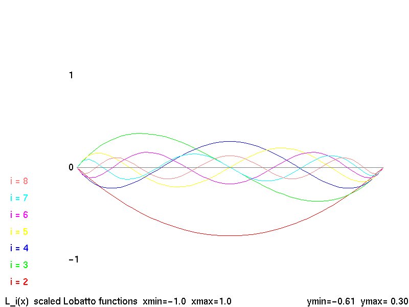 Lobatto k-2 shape functions
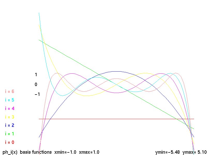 basis functions
Discretization of Triangular Grids
A very different method than FEM to solve a subset of
FEM triangle PDE's, uses discretization of a group
of points, subset of the vertices, and simultaneous
equations to get a solution.
The primary technique is the non uniform discretization of
a set of points, given in two dimensions:
nuderiv2dg.java source code
test_nuderiv2dg_tri.java test code
test_nuderiv2dg_tri_java.out test output
test_nuderiv2dg2_tri.java test code
test_nuderiv2dg2_tri_java.out test output
test_nuderiv2dg3_tri.java test code
test_nuderiv2dg3_tri_java.out test output
pde_nuderiv2dg_tri.java pde code
pde_nuderiv2dg_tri_java.out pde output
simeq.java utility class
A weaker form, note missing 'g' for general, that requires independent
points is:
nuderiv2d.java source code
test_nuderiv2d.java test code
test_nuderiv2d_java.out test output
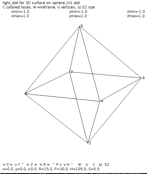
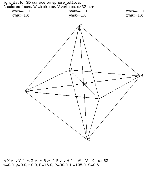
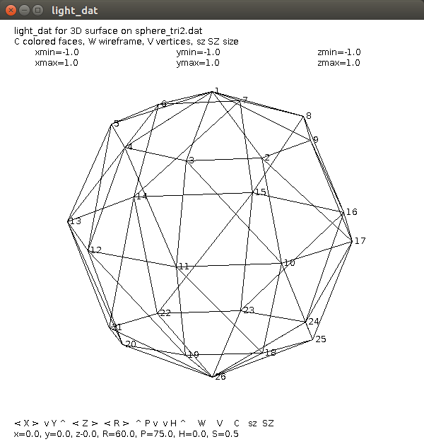
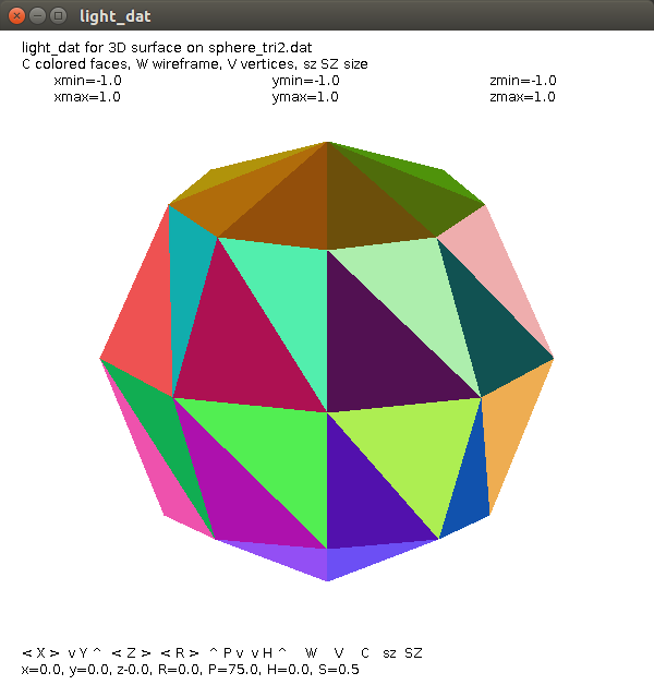
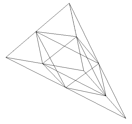
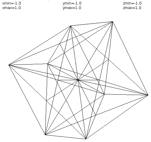
Tetrahedrons for three dimensions
Then, for three dimensions, we need tetrahedrons in place of triangles.
test_split_tetra.c test code
test_split_tetra.out test output
plot_split_tetra.c plot program
tetra_split.java utility program
test_tet_split.java test program
plot with light_dat.java source
heapsort.java source needed by light_dat
sphere_tri1.dat sphere as 8 triangles
sphere_tet1.dat sphere as 8 tetrahedrons
 sphere_tri2.dat sphere as 48 triangles
 tetra_split.dat tetrahedron split
 cube_tetra.tet cube split into tetrahedrons 4 points
cube_tetra.dat cube split into tetrahedrons 4 triangle surfaces
cube_tetra.tet cube split into tetrahedrons 4 points
cube_tetra.dat cube split into tetrahedrons 4 triangle surfaces
High order basis functions and integration
pde2sin_la.adb code, sin(x-y) 0 to 4Pi
pde2sin_la_ada.out output
pde2sin4_la.dat data for plot

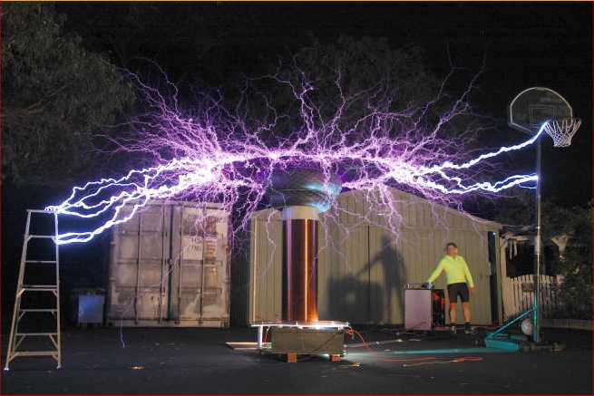
Challenging Modeling and Simulation
Solving Maxwell's equations for electric fields can be
very challenging. I have not been able to numerically
compute the discharge pattern shown below.
 Maxwell's Equations

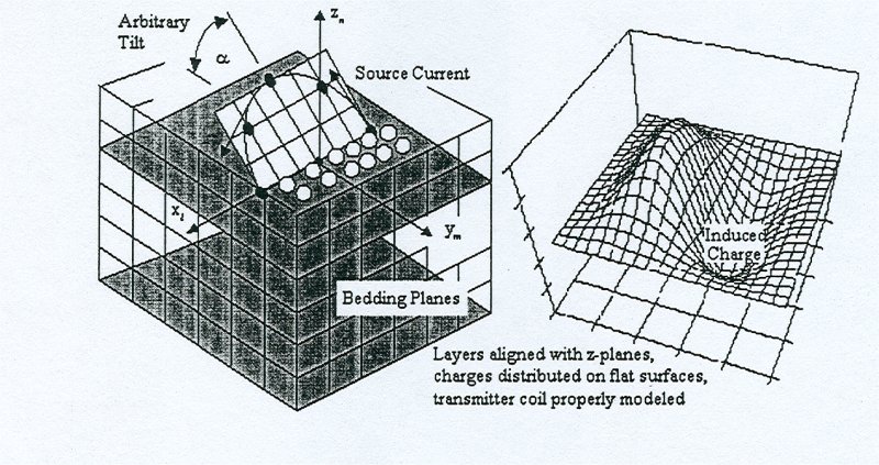 The numerical solution of Maxwell's Equations for electro-magnetic
fields may use a large four dimensional array with dimensions
X, Y, Z, T. Three spatial dimensions and time.
The numerical solution of Maxwell's Equations for electro-magnetic
fields may use a large four dimensional array with dimensions
X, Y, Z, T. Three spatial dimensions and time.
<- previous index next ->
-
CMSC 455 home page
-
Syllabus - class dates and subjects, homework dates, reading assignments
-
Homework assignments - the details
-
Projects -
-
Partial Lecture Notes, one per WEB page
-
Partial Lecture Notes, one big page for printing
-
Downloadable samples, source and executables
-
Some brief notes on Matlab
-
Some brief notes on Python
-
Some brief notes on Fortran 95
-
Some brief notes on Ada 95
-
An Ada math library (gnatmath95)
-
Finite difference approximations for derivatives
-
MATLAB examples, some ODE, some PDE
-
parallel threads examples
-
Reference pages on Taylor series, identities,
coordinate systems, differential operators
-
selected news related to numerical computation