<- previous index next ->
Numerical differentiation is typically considered poor at best.
In general, high order techniques are needed to get reasonable
values.
Similar to numerical integration, the more values of the function
that are used, then the more accuracy can be expected.
Similar to numerical integration, given a function that can be
fit accurately by an n th order polynomial, an equation for
the derivative exists to give very good accuracy.
Consider a function f(x) that you can compute but do not know
a symbolic representation. To find the derivatives at a few points,
say 4 for example, and computing only 4 evaluations of f(x):
f(x2)
* f(x3)
| *
f(x1) | |
* | |
| | |
f(x0) | | |
* | | |
| | | |
| | | |
x0 x1 x2 x3 h = x3-x2 = x2-x1 = x1-x0
We use f'(x0) to represent the derivative of f(x) at x0.
We looked up the formulas for computing the first derivative
using four equally spaced points, and write the equations:
f'(x0) = 1/6h (-11 f(x0) +18 f(x1) -9 f(x2) 2 f(x3) )
f'(x1) = 1/6h ( -2 f(x0) -3 f(x1) 6 f(x2) -1 f(x3) )
f'(x2) = 1/6h ( 1 f(x0) -6 f(x1) 3 f(x2) 2 f(x3) )
f'(x3) = 1/6h ( -2 f(x0) +9 f(x1) -18 f(x2) 11 f(x3) )
The error estimate is 1/h^4 f''''(z) for worse z in x0..x3
Thus, if the four points are fit by a third degree polynomial,
f''''(z), the fourth derivative is always zero and the numerical
derivatives are exact within roundoff error.
The values will be in an array cx[0]..[3] 1/6h*(-11, 18, -9, 2) .
Then f'(x0) = sum i=0..3 cx[i]*f(x[i])
To check that the coefficients such as -11 18 -9 2 are correct,
we symbolically fit the 4 points with a third order polynomial,
then symbolically take the derivatives. Too much work to do by
hand, thus I used Maple to check and found the coefficients correct.
Using 5 evaluations of f(x) provides the five derivatives:
f'(x0) = 1/12h (-25 f(x0) 48 f(x1) -36 f(x2) 16 f(x3) -3 f(x4) )
f'(x1) = 1/12h ( -3 f(x0) -10 f(x1) 18 f(x2) -6 f(x3) 1 f(x4) )
f'(x2) = 1/12h ( 1 f(x0) -8 f(x1) 0 f(x2) 8 f(x3) -1 f(x4) )
f'(x3) = 1/12h ( -1 f(x0) 6 f(x1) -18 f(x2) 10 f(x3) 3 f(x4) )
f'(x4) = 1/12h ( 3 f(x0) -16 f(x1) 36 f(x2) -48 f(x3) 25 f(x4) )
The above were typed by hand and could have an error.
Some quick checking: If all function evaluations are the same,
then the function is flat and the derivative must be zero at
all points. Thus, the sum of the coefficients must be zero for
every derivative. Note that the first and last coefficients have
the same values, in reverse order with reverse sign.
We will call the "12" in 1/12h the variable b or bb.
We will call the coefficients "-12", "48", "-36" the 'a' array
Always try to cut-and-paste from the computer printout:
Tabulation to compute derivatives at various points
First through sixth order, various number of points
nderiv.out
The above was generated by any of the computer programs listed below:
nderiv.c computes these cases.
nderiv.f90 in Fortran 95
nderiv.adb in Ada 95
nderiv.java in Java
deriv.py in Python 2
rderiv.py in Python 2
nderiv.py in Python 2
deriv.py3 in Python 3
Deriv.scala in Scala
deriv.go in Go language
deriv.jl in Julia
Note that the coefficients can be generated in your program by
copying the function deriv and calling it for a specific
derivative order, number of evaluations and point where derivative
is to be computed. For the second derivative using 4 evaluations
and computing the derivative at point zero,
deriv( 2, 4, 0, a, &bb); returns a={2, -5, 4, -1) and bb=1
thus f''(x0) = 1/bb h^2 ( a[0] f(x0) + a[1] f(x1) + a[2] f(x2) + a[3] f(x3) )
or f''(x0) = 1/h^2 (2 f(x0) -5 f(x0+h) +4 f(x0+2h) -1 f(x0+3h) )
deriv.h header for three versions.
deriv.c computes values.
Note that integers are returned and should be cast to appropriate
floating point type. Various languages require minor changes in the call.
This computation of derivatives will be used extensively in the
lectures that follow on ordinary and partial differential equations.
For non uniformly spaced x values, the program nuderiv.c
demonstrates how to compute the coefficients of f(x0), f(x1), ...
Note that the function nuderiv must be called in the application because
the coefficients depend on the specific problems x values.
The development for non uniformly spaced derivative coefficients is:
given x0, x1, x2, x3 non uniformly spaced
find the coefficients of y0, y1, y2, y3 y0 = f(x0) ...
in order to compute the derivatives:
y'(x0) = c00*y0 + c01*y1 + c02*y2 + c03*y3
y'(x1) = c10*y0 + c11*y1 + c12*y2 + c13*y3
y'(x2) = c20*y0 + c21*y1 + c22*y2 + c23*y3
y'(x3) = c30*y0 + c31*y1 + c32*y2 + c33*y3
Method: fit data to y(x) = a + b*x + c*x^2 + d*x^3
y'(x) = b + 2*c*x + 3*d*x^2
y''(x) = 2*c + 6*d*x
y'''(x) = 6*d
with y0, y1, y2 and y3 variables:
y0 y1 y2 y3
form: | 1 x0 x0^2 x0^3 1 0 0 0 | = a
| 1 x1 x1^2 x1^3 0 1 0 0 | = b
| 1 x2 x2^2 x2^3 0 0 1 0 | = c
| 1 x3 x3^2 x3^3 0 0 0 1 | = d
reduce | 1 0 0 0 a0 a1 a2 a3 | = a
| 0 1 0 0 b0 b1 b2 b3 | = b
| 0 0 1 0 c0 c1 c2 c3 | = c
| 0 0 0 1 d0 d1 d2 d3 | = d
this is just the inverse
y'(x0) = b0*y0 + b1*y1 + b2*y2 + b3*y3 +
2*c0*y0*x0 + 2*c1*y1*x0 + 2*c2*y2*x0 + 2*c3*y3*x0 +
3*d0*y0*x0^2 + 3*d1*y1*x0^2 + 3*d2*y2*x0^2 + 3*d3*y3*x0^2
or c00 = b0 + 2*c0*x0 + 3*d0*x0^2
c01 = b1 + 2*c1*x0 + 3*d1*x0^2
c02 = b2 + 2*c2*x0 + 3*d2*x0^2
c03 = b3 + 2*c3*x0 + 3*d3*x0^2
y'(x0) = c00*y0 + c01*y1 + c02*y2 +c03*y3 where y0 is f(x0) etc.
y'(x1) = b0*y0 + b1*y1 + b2*y2 + b3*y3 +
2*c0*y0*x1 + 2*c1*y1*x1 + 2*c2*y2*x1 + 2*c3*y3*x1 +
3*d0*y0*x1^2 + 3*d1*y1*x1^2 + 3*d2*y2*x1^2 + 3*d3*y3*x1^2
or c10 = b0 + 2*c0*x1 + 3*d0*x1^2
c11 = b1 + 2*c1*x1 + 3*d1*x1^2
c12 = b2 + 2*c2*x1 + 3*d2*x1^2
c13 = b3 + 2*c3*x1 + 3*d3*x1^2
cij = bj + 2*cj*xi + 3*dj*xi^2
y'(x1) = c10*y0 + c11*y1 + c12*y2 +c13*y3
y''(x0) = 2*c0*y0 + 2*c1*y1 + 2*c2*y2 + 2*c3*y3 +
6*d0*y0*x0 + 6*d1*y1*x0 + 6*d2*y2*x0 + 6*d3*y3*x0
or c00 = 2*c0 + 6*d0*x0
c01 = 2*c1 + 6*d1*x0
c02 = 2*c2 + 6*d2*x0
c03 = 2*c3 + 6*d3*x0
y'''(x0) = 6*d0*y0 + 6*d1*y1 + 6*d2*y2 + 6*d3*y3
or c00 = 6*d0 independent of x
c01 = 6*d1
c02 = 6*d2
c03 = 6*d3
The function prototype is
nuderiv.h
void nuderiv(int order, int npoint, int point, double x[], double c[])
where order is the order of the desired derivative
where npoint is the desired number of points (length of x[] and c[] arrays)
where point is desired x index for the derivative
where x[] is input x0, x1, ...
where c[] is output c_point_0, c_point_1, ...
For reasonably smooth functions, using larger numbers of points
allows greater spacing between points and thus fewer equations in
the system of equations to be solved.
Intermediate points may then be found by multidimensional interpolation.
See Lecture 4 for method.
nuderiv.c
nuderiv.h
nuderiv_test.c
nuderiv_test.out
nuderiv.adb
nuderiv_test.adb
nuderiv_test_ada.out
inverse.adb
nuderiv_test_exp.adb
nuderiv_test_exp_ada.out
nuderiv.f90
nuderiv_test.f90
nuderiv_test_f90.out
inverse.f90
nuderiv.java
nuderiv_test.java
nuderiv_test_java.out
test_nuderiv.java
test_nuderiv_java.out
nuderiv.py
nuderiv_test.py
nuderiv_test_py.out
Deriv.scala
TestDeriv.scala
TestDeriv_scala.out
some definitions and explanation of formulas
A test application of nuderiv.c on a 2D PDE that should be exact is
pdenu22_eq.c
pdenu22_eq.out
A test application of nuderiv.adb on a 2D PDE that should be exact is
pdenu22_eq.adb
pdenu22_eq_ada.out
A test application of nuderiv.java on a 2D PDE that should be exact is
pdenu22_eq.java
pdenu22_eq_java.out
A test application of nuderiv.f90 on a 2D PDE that should be exact is
pdenu22_eq.f90
pdenu22_eq_f90.out
A non perfect application to a smooth function exp(x*y)*sin(x+y)
pdenu_eq.c
pdenu_eq.out
pdenu_eq.adb
pdenu_eq_ada.out
pdenu_eq.java
pdenu_eq_java.out
pdenu_eq.f90
pdenu_eq_f90.out
A test application of nuderiv.c on a 3D PDE that should be close is
Note how each term of the differential equation is processed.
This case used 1.0, 2.0, ... for coefficients yet any expression
in x,y,z could be used. A term such as u(x,y,z) * du(x,y,z)/dx
would create a non linear system of equations that would be very
difficult to solve.
pdenu23_eq.c
pdenu23_eq.out
A test application of nuderiv.adb on a 3D PDE that should be close is
pdenu23_eq.adb
pdenu23_eq_ada.out
A test application of nuderiv.f90 on a 3D PDE that should be close is
pdenu23_eq.f90
pdenu23_eq_f90.out
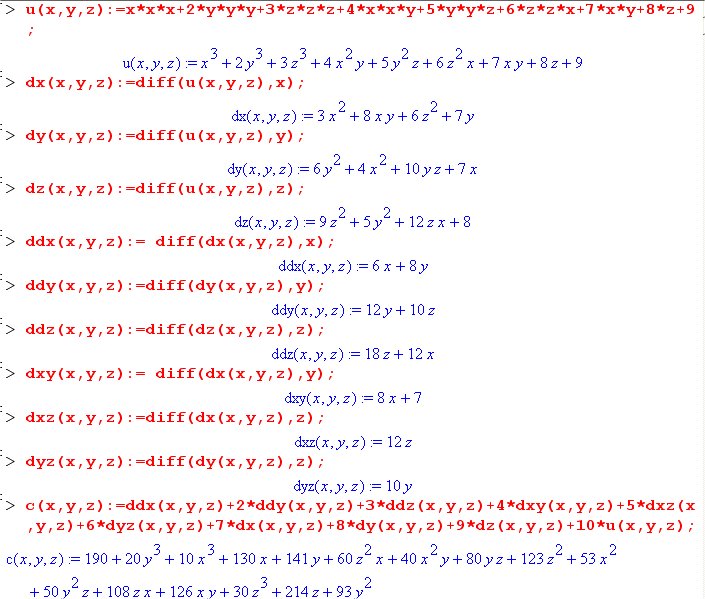
The test code was generated with Maple:
Start by choosing a solution, u(x,y,z) any function of x,y,z.
Symbolically compute the derivatives.
c(x,y,z) is computed as the RHS (right hand side) of the
chosen differential equation, dx(x,y,z) = du(x,y,z)/dx etc.
 For analytic derivatives see:
derivative.shtml
For analytic derivatives see:
derivative.shtml
<- previous index next ->
-
CMSC 455 home page
-
Syllabus - class dates and subjects, homework dates, reading assignments
-
Homework assignments - the details
-
Projects -
-
Partial Lecture Notes, one per WEB page
-
Partial Lecture Notes, one big page for printing
-
Downloadable samples, source and executables
-
Some brief notes on Matlab
-
Some brief notes on Python
-
Some brief notes on Fortran 95
-
Some brief notes on Ada 95
-
An Ada math library (gnatmath95)
-
Finite difference approximations for derivatives
-
MATLAB examples, some ODE, some PDE
-
parallel threads examples
-
Reference pages on Taylor series, identities,
coordinate systems, differential operators
-
selected news related to numerical computation