<- previous index next ->
Extending derivative computation to partial derivatives uses
the previous work on computing derivatives. Here we consider
the Cartesian coordinate system in 2, 3, and 4 dimensions,
computing second, third and fourth partial derivatives
The algorithms and some code shown below will be used when the
function is unknown, when we are solving partial differential
equations.
Consider a function f(x,y) that you can compute but do not know
a symbolic representation. To find the derivatives at a point
(x,y) we will use our previously discussed "nuderiv" nonuniform
derivative function.
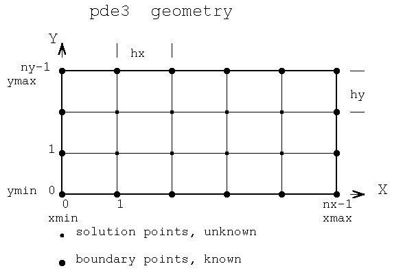
To compute the numerical derivatives of f(x,y) at a set of points
we choose the number of points in the x and y directions, nx, ny.
Thus we have a grid of cells typically programmed as a
two dimensional array.
 The partial derivative with respect to x at any (x1,y1) point
just uses points (x0,y1) (x1,y1) (x2,y1) ... (xn,y1))
The partial derivative with respect to y at any (x1,y1) point
just uses points (x1,y0) (x1,y1) (x1,y2) ... (x1,yn))
Similarly for second, third, fourth derivatives.
The partial derivative with respect to x and y is more complicated.
We first take the derivative with respect to x, same as calculus.
But, numerically, we need the value for every y.
Then, as in calculus, we take the derivative with respect to y
of the previously computed derivative with respect to x.
(Typically we save the x derivatives as a matrix because we
typically need all the partial derivatives with respect to y.)
A code fragment could look like:
static int nx = 11; /* includes boundary */
static int ny = 10; /* includes boundary */
static double xg[11] = {-1.0, -0.9, -0.8, -0.6, -0.3, 0.0,
0.35, 0.65, 0.85, 1.0, 1.2};
static double yg[10] = {-1.1, -1.0, -0.9, -0.6, -0.2,
0.3, 0.8, 1.0, 1.2, 1.3};
/* nx-2 by ny-2 internal, non boundary cells */
static double cx[11];
static double cy[10];
static double cxy[11][10]; // d^2 u(x,y)/dx dy or Uxy
for(i=1; i<nx-1; i++)
{
for(j=1; j<ny-1; j++) // computing inside boundary
{
/* d^2 u(x,y)/dxdy */
nuderiv(1,nx,i,xg,cx);
nuderiv(1,ny,j,yg,cy);
for(kx=0; k<nx; kx++)
{
for(ky=0; k<ny; ky++)
{
cxy[kx][ky] = cx[kx] * cy[ky]; // numerical derivative at each point
}
}
}
} // have cxy inside the boundary
∂2f(x,y)/∂x ∂y at x=xg[i] y=yg[i] is
computed using coefficients
cxy[kx][ky] = ∂{∂f(x,y)/∂x}/∂y * cx[kx] * cx[ky]
The partial derivative with respect to x at any (x1,y1) point
just uses points (x0,y1) (x1,y1) (x2,y1) ... (xn,y1))
The partial derivative with respect to y at any (x1,y1) point
just uses points (x1,y0) (x1,y1) (x1,y2) ... (x1,yn))
Similarly for second, third, fourth derivatives.
The partial derivative with respect to x and y is more complicated.
We first take the derivative with respect to x, same as calculus.
But, numerically, we need the value for every y.
Then, as in calculus, we take the derivative with respect to y
of the previously computed derivative with respect to x.
(Typically we save the x derivatives as a matrix because we
typically need all the partial derivatives with respect to y.)
A code fragment could look like:
static int nx = 11; /* includes boundary */
static int ny = 10; /* includes boundary */
static double xg[11] = {-1.0, -0.9, -0.8, -0.6, -0.3, 0.0,
0.35, 0.65, 0.85, 1.0, 1.2};
static double yg[10] = {-1.1, -1.0, -0.9, -0.6, -0.2,
0.3, 0.8, 1.0, 1.2, 1.3};
/* nx-2 by ny-2 internal, non boundary cells */
static double cx[11];
static double cy[10];
static double cxy[11][10]; // d^2 u(x,y)/dx dy or Uxy
for(i=1; i<nx-1; i++)
{
for(j=1; j<ny-1; j++) // computing inside boundary
{
/* d^2 u(x,y)/dxdy */
nuderiv(1,nx,i,xg,cx);
nuderiv(1,ny,j,yg,cy);
for(kx=0; k<nx; kx++)
{
for(ky=0; k<ny; ky++)
{
cxy[kx][ky] = cx[kx] * cy[ky]; // numerical derivative at each point
}
}
}
} // have cxy inside the boundary
∂2f(x,y)/∂x ∂y at x=xg[i] y=yg[i] is
computed using coefficients
cxy[kx][ky] = ∂{∂f(x,y)/∂x}/∂y * cx[kx] * cx[ky]
<- previous index next ->
-
CMSC 455 home page
-
Syllabus - class dates and subjects, homework dates, reading assignments
-
Homework assignments - the details
-
Projects -
-
Partial Lecture Notes, one per WEB page
-
Partial Lecture Notes, one big page for printing
-
Downloadable samples, source and executables
-
Some brief notes on Matlab
-
Some brief notes on Python
-
Some brief notes on Fortran 95
-
Some brief notes on Ada 95
-
An Ada math library (gnatmath95)
-
Finite difference approximations for derivatives
-
MATLAB examples, some ODE, some PDE
-
parallel threads examples
-
Reference pages on Taylor series, identities,
coordinate systems, differential operators
-
selected news related to numerical computation