SciAgents is an implementation of the MPSE approach and architecture, see [1] for a complete description of its implementation. We first discuss how solving composite PDE models fits into our MPSE approach using solvers and mediator agents. When the model of a phenomenon is simple enough, then the resulting PDE problem consists of a single domain with a single PDE defined on it (together with appropriate boundary conditions and initial conditions). There exist general solvers (PSEs) for this class of problems like //ELLPACK [2, 5]. Multiple-domain PDE problems, however, often have complicated geometry and are highly non-homogeneous, and usually require variable grid density and different discretization methods in different subdomains. Clearly, custom software is required for solving each multiple-domain PDE problem and it is not feasible to build it with traditional software development technologies. On the other hand, it is easy to observe that if the composite model can be broken down into a collection of single-domain problems, we can apply the MPSE approach.
The main issue is what mediation schemes can be applied in this case -- in other words, how to obtain a global solution out of the local solutions produced by the single-domain solvers. To do this, we use the interface relaxation technique [1, 3]. Important mathematical questions of the convergence of the method, the behavior of the solution in special cases, etc., are addressed in [4]. Typically, for second order PDEs, there are two physical or mathematical conditions involving values and normal derivatives of the solutions on the neighboring subdomains. The interface relaxation technique is as follows.
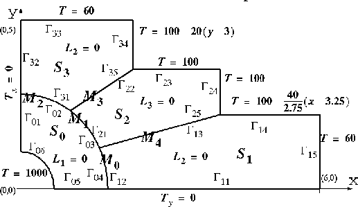
We describe the simulation of a multiple domain PDE model using four
solvers and five mediators. It models the heat distribution in the
walls of a chemical or a nuclear reactor and in the surrounding
isolating and cooling structures, see Figure 4. The
subdomains are shown, with the solver agents
![]() simulating the local process in each
subdomain and the mediators
simulating the local process in each
subdomain and the mediators ![]() mediating the
interface piece they are written on. The unknown
function is T and the exterior boundary conditions are
shown next to the corresponding boundary pieces. The reactor keeps the
inside temperature of its wall at 1000 degrees and the outside walls of the
cooling structures are kept at, more or less, room temperature. The
boundary conditions along the x and y axes reflect the symmetry of
the construction.
We denote by
mediating the
interface piece they are written on. The unknown
function is T and the exterior boundary conditions are
shown next to the corresponding boundary pieces. The reactor keeps the
inside temperature of its wall at 1000 degrees and the outside walls of the
cooling structures are kept at, more or less, room temperature. The
boundary conditions along the x and y axes reflect the symmetry of
the construction.
We denote by
![]() the k-th boundary piece of the i-th subdomain.
The differential operators
the k-th boundary piece of the i-th subdomain.
The differential operators ![]() are
are

The parameters are: ![]() ,
,
![]() ,
, ![]() ,
, ![]() ,
, ![]() .
We denote by
.
We denote by ![]() the subdomain associated with
the subdomain associated with
![]() . We use as interface conditions the continuity
of temperature and heat flow across the subdomain interfaces.
Note that even though the interface between
. We use as interface conditions the continuity
of temperature and heat flow across the subdomain interfaces.
Note that even though the interface between ![]() and
and
![]() ,
, ![]() , and
, and ![]() looks like a single curve from
the point of view of
looks like a single curve from
the point of view of ![]() , it is divided into three pieces
, it is divided into three pieces ![]() ,
,
![]() and
and ![]() , so that the mediators
, so that the mediators ![]() ,
, ![]() ,
and
,
and ![]() can each be assigned a single piece to mediate. The time
we spent from writing down the problem on paper to getting a contour
plot of the solution on screen was 5 hours (this includes some manual
calculations and adjusting the relaxation formulas for
better convergence).
can each be assigned a single piece to mediate. The time
we spent from writing down the problem on paper to getting a contour
plot of the solution on screen was 5 hours (this includes some manual
calculations and adjusting the relaxation formulas for
better convergence).

Figure 4: A sketch of a multiple domain PDE problem modeling
the heat distribution in the
walls of a chemical or a nuclear reactor and in the surrounding
isolating and cooling structures.
The subdomains are shown, with the solver agents
![]() simulating the local process in each
subdomain and the mediators
simulating the local process in each
subdomain and the mediators ![]() mediating the
interface piece they are written on. The unknown
function is T and the exterior boundary conditions are
shown next to the corresponding boundaries. We have denote by
mediating the
interface piece they are written on. The unknown
function is T and the exterior boundary conditions are
shown next to the corresponding boundaries. We have denote by
![]() the k-th boundary piece of the i-th subdomain.
the k-th boundary piece of the i-th subdomain.
A user begins solving this problem by drawing Figure 4. The sketch identifies the subdomains (the solvers), the mediators, each boundary piece in every subdomain, and the endpoints of the interfaces. The sketch is necessary since the current version of SciAgents requires input as a script file. However, we believe that (with the possible exception of the boundary piece identifiers) such a sketch will be necessary even with the best imaginable graphical user interface. We only expect the user to annotate this initial sketch.

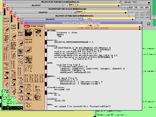
Figure 5: Four copies of the //ELLPACK interface are presented to the
user for defining the four PDE subproblems.

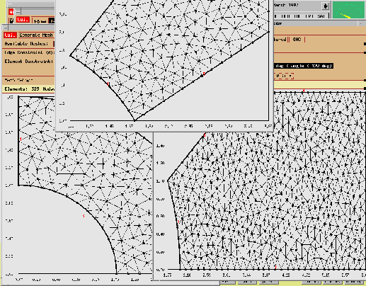
Figure 6: A snapshot of the display during the subproblem definition
process. Parts of three //ELLPACK domain tools containing three of the
subdomain geometries and finite element meshes are visible. The user
can discretize
each subdomain completely independently from the others. For example,
the densities of the above meshes are different.
After constructing the sketch the user constructs the SciAgents input file and starts SciAgents. This starts the global controller (containing the agent instantiator) and it instantiates the agents on the appropriate machines and builds the network of four solvers and five mediators that is to solve the problem. After that, the ``computing'' thread of the global controller starts a shell-like interface with two major commands: pause and tolerance for control and steering the computations. The pause prompts the controller to issue messages to all agents to save their current state and to exit. The tolerance command changes dynamically the tolerance of a given mediator or of all mediators.
After the initial exchange of of data to check that all agents are
ready, the user sees
four copies of the //ELLPACK user interface (see Figure
5). All four subproblems are
defined (see Figure 6 for a snapshot during this process)
and selecting a discretizer, linear
solver, etc., in one
subdomain does not lead to any requirement or necessity about
selections in the neighboring subdomains. If a subdomain is huge, one
may choose to use a 32-node Intel Paragon for it, while the
neighboring tiny subdomain may be simulated on the same host where the
wrapper is running. There are only two requirements for global
synchronization of the local definitions: each subdomain geometry has
to be input in terms of the global coordinate system (hence the need
of the coordinates of the boundary pieces in the sketch), and for each
interface piece, the right-hand side of the boundary conditions has to
be the function rinterface(x,y). It is the user's
responsibility to make sure that the relaxation formulas used for each
interface piece correspond to the left-hand sides of the boundary
conditions entered in the two solver's user interfaces. For the
example, the boundary condition used at all interfaces is T =
rinterface(x,y) and the relaxation formula is (U is the solution on the
``left'' side, V is the solution on the ``right'' side; ![]() is the
normal derivative; f is a factor given below; the
formula is always applied pointwise for each
point from any solver's grid/mesh on the interface):
is the
normal derivative; f is a factor given below; the
formula is always applied pointwise for each
point from any solver's grid/mesh on the interface):
![]()
The form of the factor f is
![]() which scales the relaxation properly
(and avoids dependencies on the choice of the coordinate system) and
regulates the rate of change of the boundary conditions along the
interface from iteration to iteration by changing
which scales the relaxation properly
(and avoids dependencies on the choice of the coordinate system) and
regulates the rate of change of the boundary conditions along the
interface from iteration to iteration by changing
![]() . It is sometimes hard to predict the
``optimal'', or even the acceptable, values of
. It is sometimes hard to predict the
``optimal'', or even the acceptable, values of ![]() .
.
The user input results in writing the script for the actual future runs. The user exits the //ELLPACK interface which prompts the wrapper to collect the initial data and to send them to the mediators. They compute initial right-hand sides of the boundary conditions. After the mediators provide all necessary boundary conditions, the wrapper runs the script which, in turn, runs the executable(s). When the iteration is completed the wrapper takes over again and extracts all required data from the computed solution and sends it to the mediators, waiting for the new boundary conditions from them. Thus, at the next iteration, no new compilation and user actions are necessary, since the same script (and executable(s)) is run by the wrapper.
For this example, we had to change the factor ![]() twice
before the process began to converge, especially for mediators
twice
before the process began to converge, especially for mediators ![]() and
and ![]() . This seems to be due to the
natural singularity that occurs at the reentrant corners of the global domain
which affects the stability of the convergence.
. This seems to be due to the
natural singularity that occurs at the reentrant corners of the global domain
which affects the stability of the convergence.
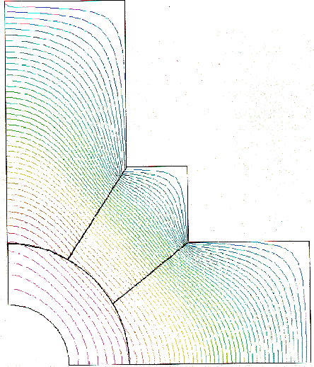
When a mediator observes convergence (the change of the boundary conditions for the next iteration is smaller than the tolerance), it reports this to the global controller, and after all mediators report convergence, the global controller issues a message to all agents to stop. In this case we had convergence after 53 iterations. Figure 7 shows a combined picture of all four subdomain solutions. Note that all contour lines match when crossing from one subdomain to another, there are even a few which go through three subdomains, and one going through all four subdomains. This is solid evidence that the interface relaxation technique works in this problem.

Figure 7: A combined picture of all subdomain solutions of the example
problem in Figure 6.1. The global solution corresponds to the physical
intuition
about the behavior of the modeled real-world system. All
contour lines match when crossing from one
subdomain to another, there are even a few which go through three
subdomains and one going through all four subdomains.