<- previous index next ->
Using Galerkin FEM on a fourth order Biharmonic PDE.
Two and three dimensions and parallel versions for C, Java, Ada and Python
Several versions of the Biharmonic PDE are used. First version is
∂4U(x,y)/∂x4 + 2 ∂4U(x,y)/∂x2∂y2 + ∂4U(x,y)/∂y4 +
2 ∂2U(x,y)/∂x2 + 2 ∂2U(x,y)/∂y2 + 2 U(x,y) = f(x,y)
First in two dimensions, then three dimensions.
Very few degrees of freedom are needed by using high order
shape functions and high order quadrature.
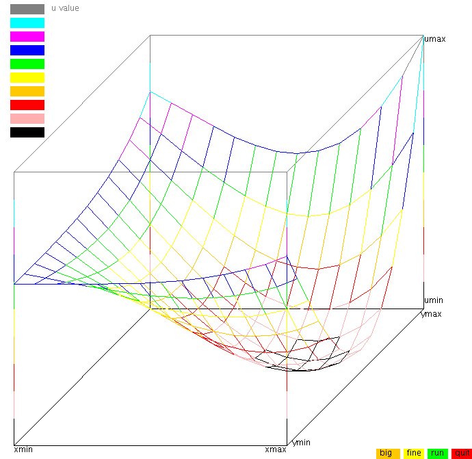
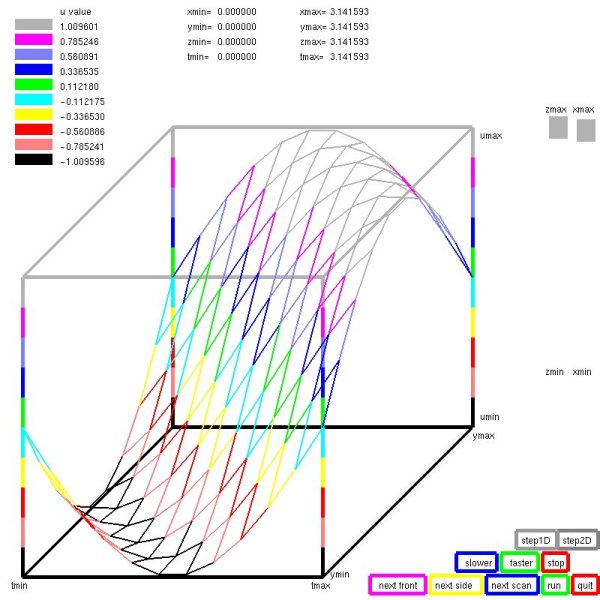
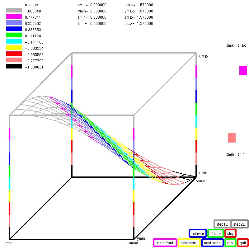
First, create test case with known solution.
Then, test that the test case is correctly coded in a language of your choice.
source code test_bihar2d.java
test output test_bihar2d.out
Plot after clicking "next" a few times.
 Next, include your test case in a PDE solver.
This case uses a previously covered Galerkin FEM with Lagrange shape functions.
Several choices higher order integration was used.
Several choices of degrees of freedom was used.
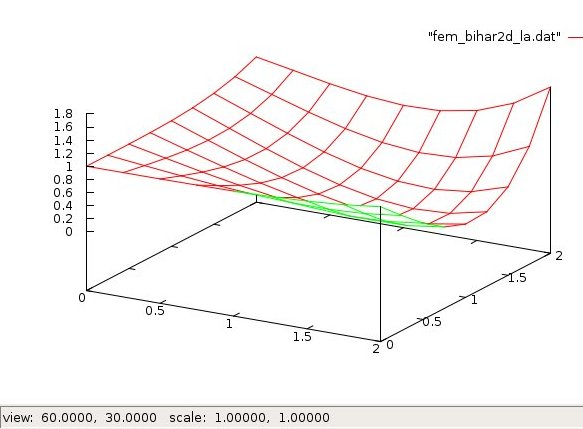
source code fem_bihar2d_la.java
output fem_bihar2d_la_java.out
source code fem_bihar2d_la.c
output fem_bihar2d_la_c.out
Plot of final solution, file plotted by gnuplot:
Next, include your test case in a PDE solver.
This case uses a previously covered Galerkin FEM with Lagrange shape functions.
Several choices higher order integration was used.
Several choices of degrees of freedom was used.
source code fem_bihar2d_la.java
output fem_bihar2d_la_java.out
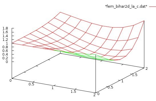
source code fem_bihar2d_la.c
output fem_bihar2d_la_c.out
Plot of final solution, file plotted by gnuplot:
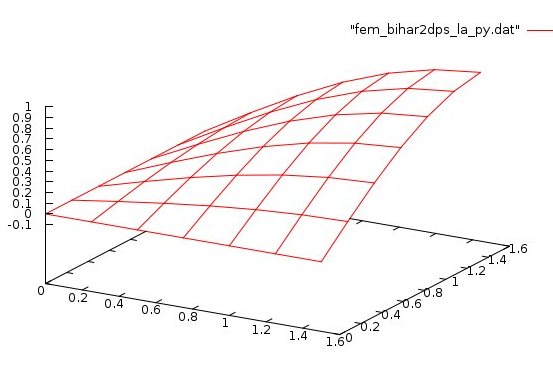
 A multi language set of fourth order biharmonic PDE solutions.
High order shape function, high order quadrature, small DOF.
Wall time and checking solution against PDE included.
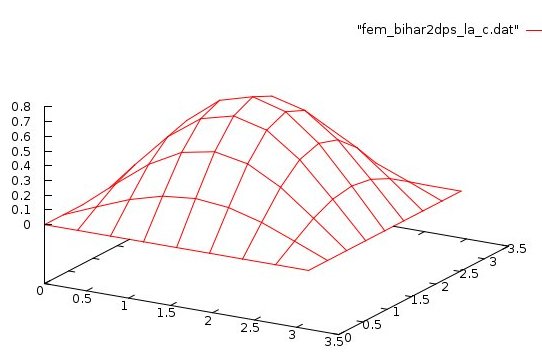
Expected solution is sin(x)*sin(y)
source code fem_bihar2dps_la.java
output fem_bihar2dps_la_java.out
source code fem_bihar2dps_la.c
output fem_bihar2dps_la_c.out
source code fem_bihar2dps_la.adb
output fem_bihar2dps_la_ada.out
source code fem_bihar2dps_la.f90
output fem_bihar2dps_la_f90.out
source code fem_bihar2dps_la.py
output fem_bihar2dps_la_py.out
A multi language set of fourth order biharmonic PDE solutions.
High order shape function, high order quadrature, small DOF.
Wall time and checking solution against PDE included.
Expected solution is sin(x)*sin(y)
source code fem_bihar2dps_la.java
output fem_bihar2dps_la_java.out
source code fem_bihar2dps_la.c
output fem_bihar2dps_la_c.out
source code fem_bihar2dps_la.adb
output fem_bihar2dps_la_ada.out
source code fem_bihar2dps_la.f90
output fem_bihar2dps_la_f90.out
source code fem_bihar2dps_la.py
output fem_bihar2dps_la_py.out
Now a three dimensional, fourth order Biharmonic PDE,
solved with few degrees of freedom and high order quadrature.
First, create test case with known solution.
Then, test that the test case is correctly coded in a language of your choice.
source code test_bihar3d.java
test output test_bihar3d.out
Plot after clicking "next" a few times.
 Next, include your test case in a PDE solver.
This case uses a previously covered Galerkin FEM with Lagrange shape functions.
Several choices higher order integration was used.
Several choices of degrees of freedom was used.
source code fem_bihar3d_la.java
output fem_bihar3d_la_java.out
source code fem_bihar3d_la.c
output fem_bihar3d_la_c.out
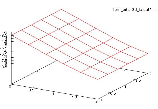
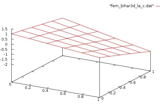
Plot of final solution at z=zmin, file plotted by gnuplot:
Next, include your test case in a PDE solver.
This case uses a previously covered Galerkin FEM with Lagrange shape functions.
Several choices higher order integration was used.
Several choices of degrees of freedom was used.
source code fem_bihar3d_la.java
output fem_bihar3d_la_java.out
source code fem_bihar3d_la.c
output fem_bihar3d_la_c.out
Plot of final solution at z=zmin, file plotted by gnuplot:
Using discretization on a fourth order Biharmonic PDE.
∂4U(x,y,z,t)/∂x4 + ∂4U(x,y,z,t)/∂y4 + ∂4U(x,y,z,t)/∂z4 + ∂4U(x,y,z,t)/∂t4 +
2 ∂2U(x,y,z,t)/∂x2 + 2 ∂2U(x,y,z,t)/∂y2 + 2 ∂2U(x,y,z,t)/∂z2 + 2 ∂2U(x,y,z,t)/∂t2 + 2 U(x,y,z,t) = f(x,y,z,t)
source code pde_bihar44t_eq.java
source code plot4d.java
output pde_bihar44t_eq_java.out
plot data pde_bihar44t_eq.dat
output plot4d.out
 Three sets of boundary for homogeneous Biharmonic PDE four dimensions
show variation in accuracy of solution.
This code writes the solution to a file for plotting with plot4d_gl.
Ada source code pde44h_eq.adb
output pde44h_eq_ada.out
Three sets of boundary for homogeneous Biharmonic PDE four dimensions
show variation in accuracy of solution.
This code writes the solution to a file for plotting with plot4d_gl.
Ada source code pde44h_eq.adb
output pde44h_eq_ada.out
 Other languages, homogeneous Biharmonic PDE in four dimensions
"C" source code pde44h_eq.c
output pde44h_eq_c.out
Fortran source code pde44h_eq.f90
output pde44h_eq_ada.f90
Java source code pde44h_eq.java
output pde44h_eq_java.out
Other languages, homogeneous Biharmonic PDE in four dimensions
"C" source code pde44h_eq.c
output pde44h_eq_c.out
Fortran source code pde44h_eq.f90
output pde44h_eq_ada.f90
Java source code pde44h_eq.java
output pde44h_eq_java.out
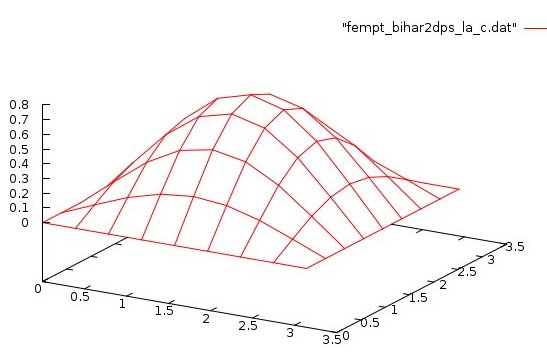
Now, make both the Java, C and Python code parallel, using threads,
Ada code parallel using tasks,
for a shared memory computer:
(coming soon for distributed memory)
source code femth_bihar2dps_la.java
output femth_bihar2dps_la_java.out
source code fempt_bihar2dps_la.c
output fempt_bihar2dps_la_c.out
source code femta_bihar2dps_la.adb
output femta_bihar2dps_la_ada.out
source code femth_bihar2dps_la.py
output femth_bihar2dps_la_py.out
 Other files, that are needed by some examples above:
Java
nderiv.java first to very high numerical derivatives
gaulegf.java low to very high order quadrature
simeq.java to about 10,000 DOF
laphi.java first through fourth order shape functions and derivatives
fem_bihar2dps_la.plot for gnuplot
femth_bihar2dps_la.plot for gnuplot
Ada
rderiv.adb first to very high numerical derivatives
deriv.adb derivative coefficients
test_deriv.adb code to check accuracy
test_deriv_ada.out accuracy limit 4th order, 11 points
gauleg.adb low to very high order quadrature
simeq.adb to about 10,000 DOF
laphi.ads first through fourth order shape functions and derivatives
laphi.adb body for above
real_arrays.ads real, real_vector, real_matrix
real_arrays.adb body for above
fem_bihar2dps_la_ada.plot for gnuplot
femta_bihar2dps_la_ada.plot for gnuplot
C
nderiv.c first to very high numerical derivatives
nderiv.h
gaulegf.c low to very high order quadrature
gaulegf.h
simeq.c to about 10,000 DOF
simeq.h
laphi.c first through fourth order shape functions and derivatives
laphi.h
fem_bihar2dps_la_c.plot for gnuplot
femth_bihar2dps_la_c.plot for gnuplot
Fortran
nderiv.f90 first to very high numerical derivatives
gaulegf.f90 low to very high order quadrature
simeq.f90 to about 10,000 DOF
laphi.f90 first through fourth order shape functions and derivatives
fem_bihar2dps_la_f90.plot for gnuplot
Python
deriv.py first to very high numerical derivatives
gauleg.py low to very high order quadrature
simeq.py to about 10,000 DOF
laphi.py first through fourth order shape functions and derivatives
pybarrier.py for parallel threads
fem_bihar2dps_la_py.plot for gnuplot
femth_bihar2dps_la_py.plot for gnuplot
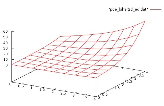
Using discretization, more difficult to program, yet faster
Works for non uniform grid in both X and Y
pde_bihar2d_eq.java very fast
simeq.java very accurate for reasonable DOF
nuderiv.java very accurate for reasonable grid
pde_bihar2d_eq_java.out output
pde_bihar2d_eq.dat output data
pde_bihar2d_eq.plot plot
pde_bihar2d_eq.sh plot
 pde_bihar2d_eq.c very fast
simeq.c
nuderiv.c
pde_bihar2d_eq_c.out output
pde_bihar2d_eq_c.plot plot
pde_bihar2d_eq.c very fast
simeq.c
nuderiv.c
pde_bihar2d_eq_c.out output
pde_bihar2d_eq_c.plot plot
A difficult first order PDE in 4 dimensions
pde4sin_eq.adb
pde4sin_eq_ada.out
pde4sin_eq.dat
Another fourth order PDE
Kuramoto-Sivashinsky equation, is shown in Lecture 31b
More fourth order PDE
The Euler Bernoulli Beam Equation (static)
∂2w/∂x2 ( E I ∂2w/∂x2 ) = q
With EI constant
∂4w/∂x4 = q(x)
The Euler Lagrange Beam Equation (dynamic)
∂2w/∂x2 ( E I ∂2w/∂x2 ) = -μ ∂2w/∂t2 = q(x,t)
can be four independent variables w(x,y,x,t)
Many methods are needed for various PDE's
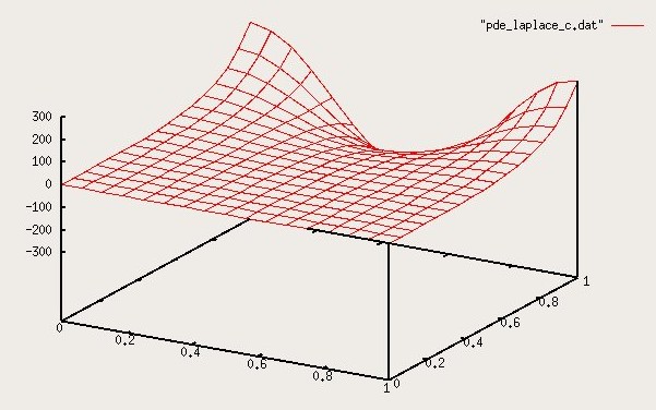
The Laplace Equation
∂2U/∂x2 + ∂2U/∂y2 = 0
Given the boundary conditions for 17 vertices in X and Y on
the unit square, using 17 points for derivatives, efficiently
solves U(x,y)=cos(k*x)*cosh(k*x) where k is about 2Pi.
Absolute error order 10E-5, with solution about -300 to 300
pde_laplace.c very fast
pde_laplace_c.out print output
pde_laplace_c.dat data output
pde_laplace_c.sh gnu plot
pde_laplace_c.plot plot
Another Laplace forth order, four dimension,
with parallel (thread) solution
This PDE needed 12th order discretization to obtain an
accuracy near 0.0001. Almost all of the execution time
was used solving 10,000 equations in 10,000 unknowns, DOF.
10 cores were used to keep the execution time to below
20 minutes rather than about 3 hours for a single core
execution.
∂4U(x,y,z,t)/∂x4 + ∂4U(x,y,z,t)/∂y4 + ∂4U(x,y,z,t)/∂z4 + ∂4U(x,y,z,t)/∂t4 +
2 ∂4U(x,y,z,t)/∂x2∂y2 + 2 ∂4U(x,y,z,t)/∂x2∂z2 +
2 ∂4U(x,y,z,t)/∂x2∂t2 + 2 ∂4U(x,y,z,t)/∂y2∂z2 +
2 ∂4U(x,y,z,t)/∂y2∂t2 + 2 ∂4U(x,y,z,t)/∂z2∂t2 -
16 U(x,y,z,t) = f(x,y,z,t) = 0
pde_bihar44tl_eq.c
pde_bihar44tl_eq_c.out
tsimeq.c
pde_bihar44tl_eq.adb
pde_bihar44tl_eq_ada.out
psimeq.adb
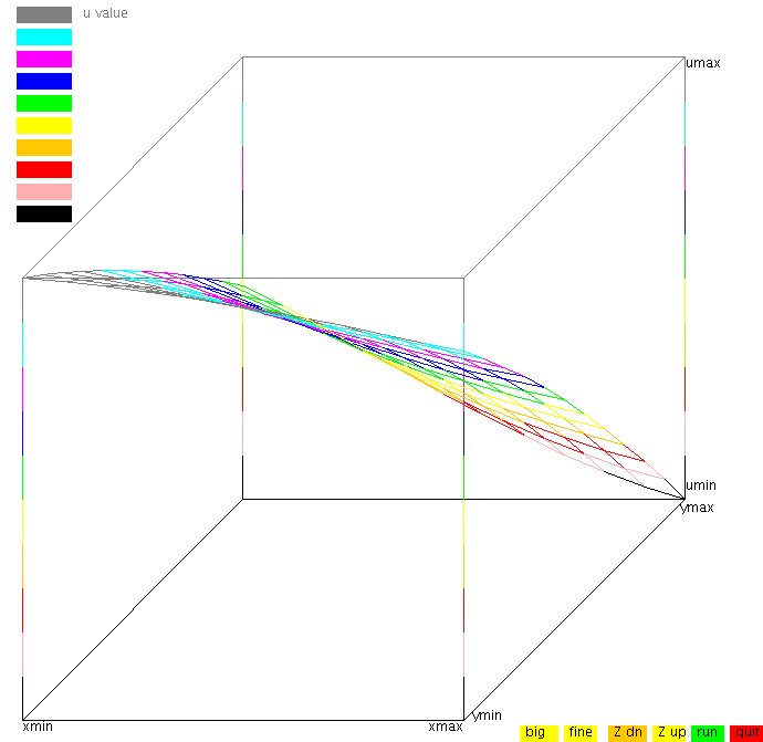
Plotted with plot4d_gl, one static view of the 4D solution is:
<- previous index next ->
-
CMSC 455 home page
-
Syllabus - class dates and subjects, homework dates, reading assignments
-
Homework assignments - the details
-
Projects -
-
Partial Lecture Notes, one per WEB page
-
Partial Lecture Notes, one big page for printing
-
Downloadable samples, source and executables
-
Some brief notes on Matlab
-
Some brief notes on Python
-
Some brief notes on Fortran 95
-
Some brief notes on Ada 95
-
An Ada math library (gnatmath95)
-
Finite difference approximations for derivatives
-
MATLAB examples, some ODE, some PDE
-
parallel threads examples
-
Reference pages on Taylor series, identities,
coordinate systems, differential operators
-
selected news related to numerical computation