<- previous index next ->
Some of the most difficult to solve PDE's have an
"order" greater than one. These are nonlinear PDE's.
A specific problem, challenge if you prefer, is the
possibility of "non physical solutions" and
"bifurcating solutions" in addition to no possible solution.
A small change in the boundary conditions or a different
starting vector for the nonlinear solver can produce
different results with no way of knowing the result is
ambiguous.
A PDE having any product or ratio of U, Ux, Uxx, etc.
is nonlinear. In two dimensions Uxx*Uxx, Uxx*UYY, etc.
Several nonlinear PDE of interest are:
Second order, third degree:
U^2 U'' + 2 U U' + 3U = f(x)
Reciprocal nonlinear:
D U' - E(x) U'/U^2 - F U'' = f(x)
An example that can handle up to third degree nonlinear systems of
equations is shown by using a Newton iteration based on the inverse
of the Jacobian:
x_next = x_prev - J^-1 * ( A * x_prev - Y)
Java nonlinear
simeq_newton5.java basic solver
test_simeq_newton5.java test program
test_simeq_newton5_java.out test_output
on four test cases (automatic adjusting heuristic used)
A linear PDE using conventional Finite Element Method, FEM, works:
source code fem_nl11_la.java
output fem_nl11_la_java.out
A nonlinear PDE using conventional FEM does not work.
source code fem_nl12_la.java
output fem_nl12_la_java.out
(very similar, nonlinear, fails)
Discretization works on nonlinear PDE's:
source code pde_nl21.java
output pde_nl21_java.out
source code pde_nl22.java
output pde_nl22_java.out
solver simeq_newton5.java
Ada nonlinear PDE
simeq_newton5.adb basic solver
test_simeq_newton5.adb test program
test_simeq_newton5_ada.out test_output
on five test cases (automatic adjusting heuristic used)
hard coded nonlinear coefficients, non unique solution
source code pde_nl13.adb
output pde_nl13_ada.out
solver simeq_newton5.adb
automated computation of nonlinear coefficients, still non unique solution
source code pde_nl13a.adb
output pde_nl13a_ada.out
solver simeq_newton5.adb
More examples with many checks:
source code pde_nl21.adb
output pde_nl21_ada.out
source code pde_nl22.adb
output pde_nl22_ada.out
Third order PDE in 3 dimensions with 3rd degree nonlinearity.
Demonstrates use of least square fit of boundary as an
initial guess to solve nonlinear system of equations.
See Lecture 4 for lsfit.ads, lsfit.adb
source code pde_nl33.adb
output pde_nl33_ada.out
Python3 nonlinear PDE
simeq_newton5.py3 basic solver
test_simeq_newton5.py3 test program
test_simeq_newton5_py3.out test_output
test_pde_nl.py3 test program
test_pde_nl_py3.out test_output
C nonlinear
source code pde_nl13.c
output pde_nl13_c.out
solver simeq_newton5.c
header simeq_newton5.h
difficulties
The nonlinear PDE can not be solved by simple application
of Finite Element Method, covered in lecture 32.
For example, the above nonlinear PDE is not solved by:
source code fem_checknl_la.c
output fem_checknl_la_c.out
Using discretization with a nonlinear solver, such as simeq_newton5,
works accurately and efficiently.
Kuramoto-Sivashinsky nonlinear
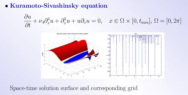 There seem to be many variations of the Kuramoto-Sivashinsky
non linear, fourth order PDE, depending on the physical problem.
I have seen in various reference papers:
Ut + Uxxxx + Uxx + 1/2 (Ux)^2 = 0 mainly variations in the last term, and
∂U(x,t)/∂t + ∂^4 U(x,t)/∂x^4 + ∂^2 U(x,t)/∂x^2 -(∂U(x,t)/∂x)^2 = 0
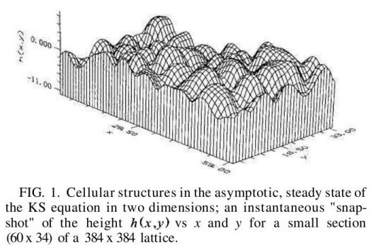
In the figure below, read h as U, read y as t.
There seem to be many variations of the Kuramoto-Sivashinsky
non linear, fourth order PDE, depending on the physical problem.
I have seen in various reference papers:
Ut + Uxxxx + Uxx + 1/2 (Ux)^2 = 0 mainly variations in the last term, and
∂U(x,t)/∂t + ∂^4 U(x,t)/∂x^4 + ∂^2 U(x,t)/∂x^2 -(∂U(x,t)/∂x)^2 = 0
In the figure below, read h as U, read y as t.
 For nonlinear PDE to be solved by solving a system of equations,
the simultaneous equations are non linear.
To solve a system of nonlinear equations reasonably efficiently,
use a Jacobian matrix and an iterative solution and adaptive
solver such as simeq_newton5, available in a few languages.
For nonlinear PDE to be solved by solving a system of equations,
the simultaneous equations are non linear.
To solve a system of nonlinear equations reasonably efficiently,
use a Jacobian matrix and an iterative solution and adaptive
solver such as simeq_newton5, available in a few languages.
Two dimensional nonlinear PDE
Solve (Uxx(x,y) + Uyy(x,y))^2 = F(x,y)
expand to
Uxx(x,y)*Uxx(x,y) + 2*Uxx(x,y)*Uyy(x,y) + Uyy(x,y)*Uyy(x,y) = F(x,y)
For pde_nl22 (Uxx(x,y)+Uyy(x,y))^2 = F(x,y)
2D grid for partial differential equation grid nx by ny
Unknown U, given boundary B, for this case nx=7, ny=6.
Zero based indexing, xmin=0.0, xmax=0.6, ymin=0.0, ymax=0.4
Does not need to be uniform, this grid has hx=0.1, hy=0.08
Uk=S(i,ii)=(i-1)*ny+(ii-1)
0.0 0.1 0.2 0.3 0.4 0.5 0.6 X
ii +------+------+------+------+------+------+------+ Y
5 | B0,5 : B1,5 : B2,5 : B3,5 : B4,5 : B5,5 | B6,5 |
+------+======+======+======+======+======+------+ 0.40
4 | B0,4 | U3 | U7 | U11 | U15 | U19 | B6,4 |
+------+------+------+------+------+------+------+ 0.32
3 | B0,3 | U2 | U6 | U10 | U14 | U18 | B6,3 |
+------+------+------+------+------+------+------+ 0.24
2 | B0,2 | U1 | U5 | U9 | U13 | U17 | B6,2 |
+------+------+------+------+------+------+------+ 0.16
1 | B0,1 | U0 | U4 | U8 | U12 | U16 | B6,1 |
+------+======+======+======+======+======+------+ 0.08
0 | B0,0 : B1,0 : B2,0 : B3,0 : B4,0 : B5,0 : B6.0 |
+------+------+------+------+------+------+------+ 0.0
0 1 2 3 4 5 6 i
Source code for solution using C, with output and debugging output
source code pde_nl22.c
output pde_nl22_c.out
output with debugging pde_nl22_c.ckout
files needed to compile and link
source code simeq_newton3.h
source code simeq_newton3.c
source code deriv.h
source code deriv.c
source code invert.h
source code invert.c
Source code for solution using Java, with output and debugging output
source code pde_nl22c,java
output pde_nl22c_java.out
output with debugging pde_nl22c_java.ckout
files needed to build
source code simeq_newton3.java
source code nuderiv.java
source code invert.java
Maple used to generate analytic solution for building test case.
Maple analytic solution pde_nl22_mws.out
Note approximate quadratic convergence to solution, from output files:
solve non linear equations A * U = F
simeq_newton3 running
simeq_newton3 itr=0, prev=1e+12, residual=71032.2
simeq_newton3 itr=1, prev=71032.2, residual=17757.5
simeq_newton3 itr=2, prev=17757.5, residual=4438.85
simeq_newton3 itr=3, prev=4438.85, residual=1109.29
simeq_newton3 itr=4, prev=1109.29, residual=276.986
simeq_newton3 itr=5, prev=276.986, residual=68.9598
simeq_newton3 itr=6, prev=68.9598, residual=17.0073
simeq_newton3 itr=7, prev=17.0073, residual=4.08366
simeq_newton3 itr=8, prev=4.08366, residual=0.906544
simeq_newton3 itr=9, prev=0.906544, residual=0.164953
simeq_newton3 itr=10, prev=0.164953, residual=0.0220222
simeq_newton3 itr=11, prev=0.0220222, residual=0.00342033
simeq_newton3 itr=12, prev=0.00342033, residual=0.000446783
simeq_newton3 finished
<- previous index next ->
-
CMSC 455 home page
-
Syllabus - class dates and subjects, homework dates, reading assignments
-
Homework assignments - the details
-
Projects -
-
Partial Lecture Notes, one per WEB page
-
Partial Lecture Notes, one big page for printing
-
Downloadable samples, source and executables
-
Some brief notes on Matlab
-
Some brief notes on Python
-
Some brief notes on Fortran 95
-
Some brief notes on Ada 95
-
An Ada math library (gnatmath95)
-
Finite difference approximations for derivatives
-
MATLAB examples, some ODE, some PDE
-
parallel threads examples
-
Reference pages on Taylor series, identities,
coordinate systems, differential operators
-
selected news related to numerical computation