<- previous index next ->
A difficult numerical problem is the finding of a global minima
of an unknown function. This type of problem is called an
optimization problem because the global minima is typically
the optimum solution.
In general we are given a numerically computable function of
some number of parameters v = f(x_1, x_2, ... , x_n)
and must find the values of x_1, x_2, ... , x_n that gives
the smallest value of v. Or, by taking the absolute value,
find the values of x_1, x_2, ... , x_n that give the value
of v closest to zero.
Generally the problem is bounded and there are given maximum and
minimum values for each parameter. There are typically many
places where local minima exists. Thus, the general solution
must include a global search then a local search to find the
local minima. There is no general guaranteed optimal solution.
First consider a case of only one variable on a non differentiable
function, y = f(x) where x has bounds xmin and xmax. There may be
many local minima, valleys that are not the deepest.
* * * * *
* * * * * * * * * *
* * * * * * * * * * *
* * * ** * * *
* *
*
Global search:
Do a y=f(x) for x = xmin, x = x+dx, until x>xmax,
Save the smallest y and the x0=x for that y.
Then find the local minimum:
Consider evaluating f(x) at some initial point x0 and x0+dx.
If f(x0) < f(x0+dx) you might move to x0-dx.
if f(x0) > f(x0+dx) you might move to x0+dx+dx.
The above may be very bad choices!
Here are the cases you should consider:
Compute yl=f(x-dx) y=f(x) yh=f(x+dx) for some dx
yh y yh y yl yl
y yh yl yl yh y
yl yl y yh y yh
case 1 case 2 case 3 case 4 case 5 case6
For your next three points, always keep best x:
case 1 x=x-dx possibly dx=2*dx
case 2 x=x-dx dx=dx/2
case 3 dx=dx/2
case 4 x=x+dx dx=dx/2
case 5 dx=dx/2
case 6 x=x+dx possibly dx=2*dx
Then loop.
A simple version in Python is
optm.py
optm_py.out
optm.py running
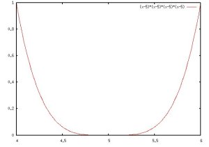
minimum (x-5)**4 in -10 to +10 initial 2, 0.001, 0.001, 200
xbest= 5.007 , fval= 2.401e-09 ,cnt= 21
minimum (x-5)**4 in -10 to +10 initial 2 using default
xbest= 4.998271 , fval= 8.9367574925e-12 ,cnt= 35
Another version, found on the web, slightly modified
min_search.py
min_search_py.out
min of (x-5)**4, h= 0.1
xmin= 4.9984375
fmin= 5.96046447754e-12
n= 86 , sx= 4.996875 , xx= 5.003125
min of (x-5)**4, h= 0.01 # smaller initial h, not as good
xmin= 4.9975
fmin= 3.90625000037e-11
n= 704 , sx= 4.995 , xx= 5.005
min of (x-5)**4, h= 2.0 # smaller tolerance, better
xmin= 4.99993896484
fmin= 1.38777878078e-17
n= 47 , sx= 4.99987792969 , xx= 5.00012207031
Beware local minima
Both of the above, will find the best of a local minima.
There could be a local minima, thus when dx gets small enough,
remember the best x and use another global search value to
look for a better optimum. Some heuristics may be needed to
increase dx. This is one of many possible algorithms.
Another algorithm that is useful for large areas in two
dimensions for z=f(x,y) is:
Use a small dx and dy to evaluate a preferred direction.
Use an expanding search, doubling dx and dy until no more
progress is made. Then use a contracting search, halving dx and dy
to find the local minima on that direction.
Repeat until the dx and dy are small enough.
The numbers indicate a possible order of evaluation of the points
(in one dimension).
1
2
3
5
6
7 Value computed
4 ^
8 |
9
------------> X direction
Numbers are sample number.
Note dx doubles for samples 2, 3, 4, 5
then dx is halved and added to best so far, 4, to get 6
then halved to get 7, 8, 9.
There may be many expansions and contractions.
The pseudo derivatives are used to find the preferred direction:
(After finding the best case from above, make positive dx and dy best.)
z=f(x,y)
zx=f(x+dx,y) zx < z
zy=f(x,y+dy) zy < z
r=sqrt(((z-zx)^2+(z-zy)^2))
dx=dx*(z-zx)/r
dy=dy*(z-zy)/r
This method has worked well on the spiral trough.
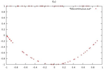
The really tough problems have many discontinuities.
I demonstrated a function that was everywhere discontinuous.
The function was f(x)=x^2-1 with f(x)=1 if the bottom bit
of x^2-1 is a one.
discontinuous.c first function
discontinuous.out
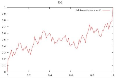
 Another, recursive, function that is continuous, yet in the
limit of recursing, nowhere differentiable, is:
double f(x){ /* needs a termination condition, e.g count=40 */
if(x<=1.0/3.0) return (3.0/4.0)*f(3.0*x);
else if(x>=2.0/3.0) return (1.0/4.0)+(3.0/4.0)*f(3.0*x-2.0);
else /* 1/3 < x < 2/3 */
return (1.0/4.0)+(1.0/2.0)*f(2.0-3.0*x);}
discontinuous.c second function
discontinuous.out
Another, recursive, function that is continuous, yet in the
limit of recursing, nowhere differentiable, is:
double f(x){ /* needs a termination condition, e.g count=40 */
if(x<=1.0/3.0) return (3.0/4.0)*f(3.0*x);
else if(x>=2.0/3.0) return (1.0/4.0)+(3.0/4.0)*f(3.0*x-2.0);
else /* 1/3 < x < 2/3 */
return (1.0/4.0)+(1.0/2.0)*f(2.0-3.0*x);}
discontinuous.c second function
discontinuous.out
 In general, it will not work to use derivatives, or even pseudo
derivatives without additional heuristics.
A sample program that works for some functions of three
floating point parameters is shown below. Then, a more general
program with a variable number of parameters is presented
with a companion crude global search program.
Two parameter optimization in Python useful for project
optm2.py3 source code
optm2_py3.out output
global_search.py3 source code
search_py3.out output
search.py3 source code
search2_py3.out output
notice that zbest stops getting better at some small dx, dy
mpmath_example.py3 source code
mpmath_example_py3.out output
test_mpmath.py3 source code
test_mpmath_py3.out output
Two parameter optimization in java
global_search.java source code
global_search_java.out output
search2.java source code
search2_java.out output
notice that zbest stops getting better at some small dx, dy
Three parameter optimization:
optm3.h
optm3.c
test_optm3.c
test_optm3_c.out
N parameter optimization in C and java:
This includes a global search routine srchn.
optmn.h
optmn.c
test_optmn.c
test_optmn_c.out
optmn_dev.java
test_optmn_dev.java
test_optmn_dev_java.out
optmn_interface.java
optmn_function.java user modifies
optmn.java
optmn_run.java
optmn_run_java.out
In MatLab use "fminsearch" see the help file.
Each search is from one staring point.
You need nested loops to try many starting points.
I got error warnings that I ignored, OK to leave them in your output.
optm.m
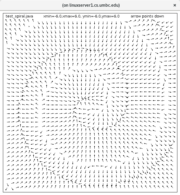
An interesting test case is a spiral trough:
In general, it will not work to use derivatives, or even pseudo
derivatives without additional heuristics.
A sample program that works for some functions of three
floating point parameters is shown below. Then, a more general
program with a variable number of parameters is presented
with a companion crude global search program.
Two parameter optimization in Python useful for project
optm2.py3 source code
optm2_py3.out output
global_search.py3 source code
search_py3.out output
search.py3 source code
search2_py3.out output
notice that zbest stops getting better at some small dx, dy
mpmath_example.py3 source code
mpmath_example_py3.out output
test_mpmath.py3 source code
test_mpmath_py3.out output
Two parameter optimization in java
global_search.java source code
global_search_java.out output
search2.java source code
search2_java.out output
notice that zbest stops getting better at some small dx, dy
Three parameter optimization:
optm3.h
optm3.c
test_optm3.c
test_optm3_c.out
N parameter optimization in C and java:
This includes a global search routine srchn.
optmn.h
optmn.c
test_optmn.c
test_optmn_c.out
optmn_dev.java
test_optmn_dev.java
test_optmn_dev_java.out
optmn_interface.java
optmn_function.java user modifies
optmn.java
optmn_run.java
optmn_run_java.out
In MatLab use "fminsearch" see the help file.
Each search is from one staring point.
You need nested loops to try many starting points.
I got error warnings that I ignored, OK to leave them in your output.
optm.m
An interesting test case is a spiral trough:
 Possibly a better view:
 test_spiral.f90
test_spiral_f90.out
spiral.f90
test_spiral.c
test_spiral_c.out
spiral.h
spiral.c
test_spiral.java
test_spiral_java.out
test_spiral.f90
test_spiral_f90.out
spiral.f90
test_spiral.c
test_spiral_c.out
spiral.h
spiral.c
test_spiral.java
test_spiral_java.out
 spiral_trough.py
test_spiral.py
test_spiral_py.out
Your project is a multiple precision minimization
See Lecture 15 for multiple precision
spiral_trough.py
test_spiral.py
test_spiral_py.out
Your project is a multiple precision minimization
See Lecture 15 for multiple precision
<- previous index next ->
-
CMSC 455 home page
-
Syllabus - class dates and subjects, homework dates, reading assignments
-
Homework assignments - the details
-
Projects -
-
Partial Lecture Notes, one per WEB page
-
Partial Lecture Notes, one big page for printing
-
Downloadable samples, source and executables
-
Some brief notes on Matlab
-
Some brief notes on Python
-
Some brief notes on Fortran 95
-
Some brief notes on Ada 95
-
An Ada math library (gnatmath95)
-
Finite difference approximations for derivatives
-
MATLAB examples, some ODE, some PDE
-
parallel threads examples
-
Reference pages on Taylor series, identities,
coordinate systems, differential operators
-
selected news related to numerical computation