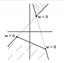
Figure 1: An example of an external triangle. Both shaded regions are part of a single external triangle.
|
Marc Olano University of North Carolina olano@cs.unc.edu |
Trey Greer Hewlett-Packard greer@chapelhill.hp.com |
Copyright (c) 1997, by ACM, Inc.
We present a new triangle scan conversion algorithm that works entirely in homogeneous coordinates. By using homogeneous coordinates, the algorithm avoids costly clipping tests which make pipelining or hardware implementations of previous scan conversion algorithms difficult. The algorithm handles clipping by the addition of clip edges, without the need to actually split the clipped triangle. Furthermore, the algorithm can render true homogeneous triangles, including external triangles that should pass through infinity with two visible sections. An implementation of the algorithm on Pixel-Planes 5 runs about 33% faster than a similar implementation of the previous algorithm.
CR Categories and Subject Descriptors: I.3.1 [Computer Graphics]: Hardware Architecture - Parallel Processing; I.3.3 [Computer Graphics]: Picture/Image Generation; I.3.7 [Computer Graphics]: Three-Dimensional Graphics and Realism - Visible line/surface algorithms.
Additional Keywords: homogeneous coordinates, scan conversion, rasterization, clipping
Homogeneous coordinates are commonly used for transformations in 3D graphics. They are popular because rotation, scaling, translation and perspective are all linear in homogeneous space. As a result, transformations can be expressed uniformly in matrix form and can be easily combined into a single composite matrix. While homogeneous coordinates are used for 3D transformations, points are converted back to true 3D after hither clipping. One of the reasons that hither clipping is required is to avoid singularities in this conversion.
We present a method for triangle scan conversion in which all computations occur in homogeneous space. In a comparison of similar implementations of the new algorithm and the previous algorithm on Pixel-Planes 5 [Fuchs89], the new algorithm ran about 33% faster.
With the new method, no hither clipping is required at all for the (rather uninteresting) case using only flat shading and no z-buffering. Even triangles that touch or cross the camera plane are rendered correctly.
A hither clip edge must be used when values are interpolated across the triangle (Z, color, texture coordinates, etc.). Even so, the algorithm never splits the triangle and does not have to compute new shading parameter values or vertex locations at the clipping plane. This is at the "cost" of having to use perspective-correct interpolation for every parameter.
The new algorithm requires more total operations, due to the perspective-correct interpolation of all parameters. However, support for these perspective-correction operations exists in current hardware. As our tests show, the algorithm can run faster on actual hardware. The computation required is more regular than previous algorithms, avoiding costly branches for clipping. The algorithm allows heavy pipelining of the transformation and setup processing, and is more amenable to hardware implementation. As most highly parallel graphics hardware systems have more processing power at the pixel level than at the transformation level, and must already handle perspective correction of texture coordinates, we expect scan conversion with 2D homogeneous coordinates to be a faster alternative on a range of hardware graphics systems.
Traditional triangle scan conversion algorithms walk along polygon edges and fill across scan lines. Pineda observed that these algorithms do not extend well to parallel implementations [Pineda88].
The Pixel-Planes [Fuchs85] and Pineda [Pineda88] scan conversion algorithms do parallelize well. In both of these algorithms, each triangle edge is represented by a linear edge function. The edge function is positive inside the edge and negative outside. Within a triangle, all of the edge functions are positive; outside the triangle, at least one edge function is negative. Both the Pixel-Planes and Pineda algorithms take advantage of the linearity of the edge functions. In the Pixel-Planes family of graphics systems, a hardware multiplier tree computes the value of each linear edge function at a large number of pixels simultaneously. In the Pineda algorithm, the value of an edge function at a pixel is computed incrementally, with a single addition, from the value at the previous pixel. Both methods compute the coefficients of the edge function from the 2D screen coordinates in the same way. For the edge between (Xi-1, Yi-1) and (Xi, Yi), the edge function Ei is computed as
|
dXi = Xi - Xi-1 |
|
dYi = Yi - Yi-1 |
|
Ei(X, Y) = (X - Xi) dXi
- (Y - Yi) dYi |
Similar equations are used to compute the coefficients for linear functions to interpolate parameters across the triangle (color, texture coordinates, etc.). Hidden in these equations are the divisions required to project each of the three vertices onto the screen and another division required to normalize the parameter interpolation equations. The new algorithm computes equivalent edge functions and parameter interpolation functions using 2D homogeneous screen coordinates without computing the actual screen coordinates.
The new algorithm can be derived from the 2D equivalent to the 3D homogeneous point-in-tetrahedron test given by Niizeki [Niizeki94]. In this test, a 3D point is in a tetrahedron if it passes four 4x4 determinant tests. That is (x, y, z, w) is in the tetrahedron defined by four points, (xi, yi, zi, wi), when these four determinants all have the same sign:
|
, , , |
We can derive a similar 2D point-in-triangle test using three 3x3 determinant tests. The result of each edge function at a pixel is equivalent to (and with the right scaling, equal to) the result of one of the determinants. The edge function form is superior for incremental evaluation. Niizeki also gives a point-in-polygon test, but it is not appropriate for our purposes as it is for 3D points in 3D polygons.
Blinn noted the possibility of scan converting without hither clipping, though he still suggested operating in non-homogeneous space for the actual scan conversion [Blinn96b].
A point in 3-space, P = (X, Y, Z), is represented in homogeneous coordinates by the four element vector, p = (X, Y, Z, 1). Any non-zero multiple of this homogeneous vector represents the same point in 3-space. Similarly, there are non-homogeneous, P = (X, Y), and homogeneous, p = (x, y, w), representations of points in 2-space. Notice that while 3D non-homogeneous and 2D homogeneous representations both have three components, they represent points in different spaces. Except when converting between representations, we will write points in non-homogeneous coordinates in upper case and points in homogeneous coordinates in lower-case. We will also use different fonts for 2D and 3D points.<\p>
To convert a non-homogeneous representation to a homogeneous representation, append a w coordinate of 1, (X, Y, Z) (X, Y, Z, 1) or (X, Y) (X, Y, 1). To convert a homogeneous representation to a non-homogeneous representation, divide each component by w, (x, y, z, w) (x/w, y/w, z/w) or (x, y, w) (x/w, y/w). This is called the projection of the homogeneous point. The representations and conversions are summarized in Table 1.
| non-homogeneous | homogeneous | |
|---|---|---|
| 2D | P = (X, Y) = (x/w, y/w) |
p = (x, y, w) = (X, Y, 1) |
| 3D | P = (X, Y, Z) = (x/w, y/w z/w) |
p = (x, y, z, w) = (X, Y, Z, 1) |
A triangle can be defined as a weighted linear combination of three vertices [Niizeki94]. In homogeneous coordinates:
| p = t0 p0 + t1 p1 + t2 p2 |
 Figure 1: An example of an external triangle. Both shaded regions are part of a single external triangle. |
(where the t's have the same sign and at least one is non-zero). This definition holds whether the points are 2D or 3D. If the w components of all three vertices have the same sign, the result is the bounded triangle we normally expect. However, if the w components do not all have the same sign, the result is an external triangle, that wraps through infinity to connect the vertices (Figure 1).
To understand the connection between 2D homogeneous triangles and 3D triangles, we will look at a single 3D triangle and its projection onto the screen. For simplicity, we will define the triangle in canonical eye space. In canonical eye space, the center of projection is at the origin, the direction of projection is aligned down the Z axis, and the field of view is 90 degrees. In this space, perspective projection can be achieved simply by dividing by Z. In other words, to project the 3D point (X, Y, Z), set x = X, y = Y, and w = Z to get the 2DH point (x, y, w). Figure 2 and Figure 3 show a triangle with two vertices in front of the eye as the Z coordinate of the third vertex changes. Figure 4 shows a triangle with one vertex in front of the eye as the Z coordinate of the other two change.
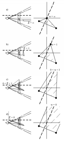
Figure 2: Views of what happens to a triangle as one of the vertices moves in Z. For each case, a side view and a view of the resulting image are shown. The heavy dashed line shows the path followed by the moving vertex. a) The top vertex is infinitely far away. It projects to the center of projection. b) The vertex is at a "normal" distance in front of the eye. c) The vertex is still in front of the eye but out of the viewing frustum. d) The vertex is even with the eye, which maps it to a point "at infinity" in the image plane. |
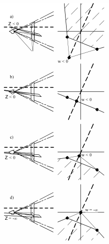
Figure 3: More views of what happens to a triangle as one of the vertices moves in Z. a) The vertex has moved behind the eye. The displayed projection is one part of an "external" triangle. b) The plane of the triangle passes through the eye, so nothing is visible. c) The triangle has passed completely through the eye, now we see the back. d) The vertex is infinitely far behind the eye. The projection of the vertex is again at the vanishing point, but we see part of an external triangle now.
|
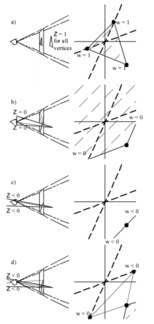
Figure 4: Views of what happens to a triangle if two vertices pass behind the eye while the other remains in front. Once again, a side view and the resulting projection are shown. The lines indicating the path of the vertices are left out of the side view for clarity, but still appear in the projected view. a) All vertices are in front of the eye. This is the same as Figure 2b. b) both vertices are in the plane of the eye. They project to infinity in different directions. c) The plane of the triangle passes through the eye so nothing is visible. d) Both vertices are behind the eye. What is visible is part of an external triangle, but the "other half" from what was visible in Figure 3a, c, and d. |
Before attacking the full scan conversion problem, consider the equations for perspective-correct interpolation across a triangle. This is called hyperbolic interpolation by Blinn [Blinn96b] and rational linear interpolation by Heckbert [Heckbert89].
If some parameter (say the u texture coordinate) is to vary linearly across the triangle in 3D (i.e. across the object itself), it must obey this equation:
| u = a X + b Y + c Z | (1) |
The 3D position (X, Y, Z) projects to 2D, using the 2D homogeneous representation (x, y, w) where x = X, y = Y, w = Z. This allows us to rewrite equation 1 to hold in 2D homogeneous space:
| u = a x + b y + c w | (2) |
Division by w produces the familiar 2D perspective-correct interpolation equation [Blinn96b, Heckbert89]:
| u/w = a x/w + b y/w + c = a X + b Y + c | (3) |
This says that u/w is a linear function in the screen space (X, Y). The coefficients a, b, and c are the same equations 1, 2 and 3. Given a value for u at each vertex (e.g. the parameter vector [u0 u1 u2]), we can solve for [a b c] using equation 2:
| [a b c] = [u0 u1 u2] = [u0 u1 u2] M-1 | (4) |
Consider the implications of this result. We can invert one 3x3 matrix, which depends only on the vertex locations before perspective projection. Then computation of the coefficients for perspective-correct interpolation requires just one 3x3 vector-matrix multiply per parameter to interpolate.
The coefficients are derived directly from the homogeneous coordinates of the vertices. Since they are based on the 2DH coordinates and not the 3D coordinates, they are independent of the 3D point representation. In particular, the parameter interpolation will still work even if the original vertices were 3D homogeneous coordinates with arbitrary w components (as might result from rational splines).
Since we never divide by w for any of the vertices, we avoid the usual troubles when w is zero or negative which necessitate costly clipping operations. The coefficient computations are independent of any clipping required for scan conversion, and do not require computation of the values of each parameter at the clip points, even if the triangle crosses behind the eye. These coefficients can be used for parameter interpolation with any scan conversion technique, either by direct evaluation of the linear expression (as is done on the Pixel-Planes hardware) or incrementally.
As this is a perspective-correct interpolation, the result at each pixel is u/w. To recover the true parameter value, it is necessary to also interpolate 1/w. Once per pixel, we take the reciprocal, then per parameter perform a multiplication of the form (u/w) * w. Coefficients for 1/w can be computed using the parameter vector [1 1 1] (giving the sum of the columns of M-1).
There are several reasons that we do not mind this extra per-pixel computation. First, perspective correction is already required for texture coordinates, including interpolation of 1/w and its reciprocal. Second, all clipping and projection are deferred from computations at the vertices, where they are difficult, to computations at the visible pixels, where they are easy. This makes both the pixel-level and transformation and setup-level processing simpler. Third, graphics hardware typically has many fewer processors devoted to transformations, clipping, and setup than pixel computations, making the efficiency of the former much more critical. Finally, our particular hardware implementation avoids most of the per-pixel costs by using deferred shading.
The coefficient computations for parameter interpolation can be extended to complete triangle scan conversion. Following the Pixel-Planes and Pineda algorithms [Fuchs85, Pineda88], we compute a linear function for each edge of the triangle. This function is positive on inside of the edge and negative on the outside. Since both the edge function and parameter interpolation functions are linear, the edge function is just a parameter interpolation function for some pseudo-parameter. For each edge, we define a pseudo-parameter that is zero at the two vertices on the edge and one at the opposite vertex. From equation 4, it is apparent that the edge parameter vectors [1 0 0], [0 1 0], and [0 0 1] simply pick rows out of the inverse matrix.
Examining the edge functions just defined and the determinant tests of [Niizeki94], we can show that they are different formulations for the same test. For the pixels in the part of the triangle we usually want to render, all of the edge functions are positive*. [* We can use this fact to create an efficient scan converter that renders triangles without every doing any clipping. All visible portions of the triangles have positive results on all of their edge functions. Whole or partial triangles behind the eye have negative results on their edge functions.]
Computation of the 3x3 matrix inverse requires division by the 3x3 determinant of M. This might cause some concern, as sometimes the matrix inverse will not exist. In 3D, a matrix determinant gives twice the signed volume of a tetrahedron. In eye space, this is the tetrahedron with the eye at the apex and the triangle to be rendered as the base. If all of the 2D w coordinates are 1, the determinant is also exactly twice the signed screen-space area of the triangle. If the determinant is zero, either the triangle is degenerate or the view is edge-on (Figure 2b and Figure 4c).
So, if the M-1 does not exist, the triangle should not be rendered anyway. Furthermore, for vertices defined by the right-hand rule, the determinant is positive if the triangle is front-facing and negative if the triangle is back-facing.
For numerical accuracy, we actually throw away triangles with sufficiently small determinants as well as the ones with zero determinants. To avoid loosing large meshes of very small triangles, we snap the 2D homogeneous coordinates of the vertices to a fine grid (you can think of this as a 3D grid in canonical eye space). This retains the mesh connectivity, but forces the small triangles to either snap to zero area or to a size large enough to render.
To add arbitrary clip planes, we compute new clip edge functions. We only need the new edge functions, we do not actually find the clip vertices. The pseudo-parameter vector for a clip edge function is just the dot product test normally used for determining which vertices are inside or outside the clip plane [Cyrus78]. It is linear, positive for unclipped points, negative for clipped points, and zero along the clipping plane itself. The parameter vector [c0 c1 c2] for a clip plane with normal N = [Nx Ny Nz] and containing the point Pc is
| [c0 c1 c2] = [Nx Ny Nz N.Pc] |
Usually, this dot product is simplified to take advantage of the known simple values of N and Pc. We use this method to create a hither edge function.
Scan conversion of the triangle edges works without clipping. We have implemented a scan converter on Pixel-Planes 5 [Fuchs89] that renders flat shaded non-z-buffered triangles with no clipping at all. Computation of coefficients for parameter interpolation also works without clipping. However, for triangles that pass near the eye, the parameter interpolation can overflow. This is true even if the parameter itself is well defined. For example, even if u doesn't overflow, u/w and 1/w may. The hither edge masks out regions where parameters might overflow.
With the use of a hither edge, our implementation is able to use fixed point to store interpolated values like 1/w. With the hither plane we can safely use the full fixed-point range, with 1/w reaching the maximum representable value exactly on the hither plane.
So far, we have only discussed perspective-correct interpolation. In fact we use only perspective-correct interpolation. In traditional scan conversion, it has been common to interpolate parameters linearly in screen space. This produces some distortions which prevent uncorrected interpolation from working for texture coordinates, but avoids the per-pixel divide required by the correction process. We can derive coefficients for uncorrected interpolation:
| u = a X + b Y + c = a x/w + b y/w + c | |
| u w = a x + b y + c w | (5) |
Equation 5 is now in same form as equation 4. Therefore, a parameter vector [u0w0 u1w1 u2w2] can be used to compute the coefficients for uncorrected interpolation. Alternately, a new matrix can be created and used for all uncorrected interpolation:
| [a b c] = [u0 u1 u2] |
Unlike perspective-correct interpolation, uncorrected interpolation does not work without explicit clipping. In any external triangle (including any triangle crosses behind the eye), we also get an external interpolation. For example, to interpolate between 0 and 1, the parameter value starts at 0, goes negative, and wraps through infinity to get to 1. To avoid this, it is necessary to do full clipping on all triangles to avoid ever rendering external triangles.
As a result, uncorrected interpolation requires more setup and complicates the setup processing. For this reason, we only use perspective-correct interpolation.
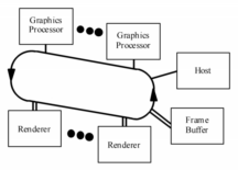
Figure 5: Pixel-Planes 5 block diagram [Fuchs89]. Graphics Processors are Intel i860 microprocessors, Renders are 128x128 custom SIMD arrays. |
As mentioned earlier, we have implemented the 2D homogeneous scan conversion algorithm on the Pixel-Planes 5 graphics system (Figure 5). Pixel-Planes 5 has a number of graphics processors, responsible for geometric transformations and rendering setup computation, and a number of renderers, responsible for scan conversion and shading. Each graphics processor uses a general purpose Intel i860 processor for geometric transformations and rendering setup computations. Each renderer has a 128x128 SIMD array with a linear expression tree capable of simultaneously evaluating the results of a linear expression across the entire 128x128 array.
Pixel-Planes 5 is a good machine to take advantage of the 2D homogeneous scan conversion algorithm. The processors it uses for transformation and setup use pipelined floating point, but are not very efficient for code with lots of branching. In fact, the algorithm would work well on a machine with an even deeper floating point pipeline. The processors it uses for rasterization include a linear expression tree, which makes evaluation of edges and interpolation functions particularly easy. They also have enough memory per-pixel (208 bits) to store all the parameters needed for shading, allowing us to use deferred shading. This means that we rasterize all of the parameters used for shading, but don't do the shading computations until all primitives have been rasterized. As a result, the reciprocal and multiplications necessary to recover the true parameter values (as well as the rest of the shading computations) are only done for the visible pixels instead of for every pixel of every primitive. Deferred shading also gives 100% utilization of the SIMD processor arrays during the perspective correction and shading computations.
Because the Pixel-Planes 5 linear expression tree evaluates expressions for all pixels in a 128x128 region, our implementation uses an extra edge normalization that would not be required in an incremental algorithm. For incremental scan conversion [Pineda88], we would only evaluate the edge functions inside or near the triangle, so the addition of a hither plane can prevent their overflow. For Pixel-Planes style scan conversion, the edge functions are evaluated at many pixels simultaneously, some of which may be far outside the triangle. This is only a concern for the edge functions, not the parameter interpolation. Parameter values outside the triangle are not used, so it doesn't matter if they overflow there.
Since only the sign of each edge function matters, we can scale each edge to avoid overflow within the screen boundaries. Any scaling factor will do, as long as it can be guaranteed to bound the range of the edge function within one screen regions. In the Pixel-Planes 5 implementation, we used the simple but somewhat expensive 1/(|a| + |b|). An optimized version would probably prefer to use a power of two scaling factor, which would require only exponent addition for floating point or shifts for fixed point representations of the edge function coefficients.
Certain anti-aliasing algorithms (not used in our implementation) require
the distance of pixels from the edge. For these, the distance can be computed
exactly, using an edge function normalized by 1/sqrt(a2 +
b
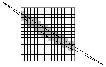
Figure 6: A hard triangle to bin correctly. An axis-aligned bounding box binner would attempt to scan convert the triangle in every region on the screen when it really only lands in the shaded regions. |
Pixel-Planes 5 uses screen-space subdivision to allocate screen area to the SIMD rendering blocks. While the algorithm behaves correctly if a renderer attempts to scan convert a triangle that does not land in its screen region, it does waste time that could be used rendering other triangles. To get maximum processor utilization, we need to make good estimates of the region coverage of each triangle. Binning is the job of finding the regions that contain part of the triangle.
For the implementation we used for performance testing, we simply used an axis-aligned bounding box around the triangle for binning. Computing bounding boxes from pre-projection homogeneous coordinates is covered by Blinn in [Blinn96a]. However, particularly for triangles with high aspect ratios, the axis aligned bounding box can seriously overestimate the number of regions covered (Figure 6). This problem is becoming more serious, as region sizes shrink to increase processor utilization.
We can compute the exact binning, while still using only homogeneous coordinates. The exact binning algorithm relies on homogeneous point-inside-edge tests and edge-edge intersection tests. The point-inside-edge test is just the edge function evaluated at the point. The edge-edge intersection test is made up of four point-inside-edge tests. The two end-points of the first edge must be on opposite sides of the second edge, while the two end-points of the second edge must be on opposite sides of the first.
A triangle intersects a region if
Since the region edges and corners are spaced evenly, all of the tests involved can be evaluated incrementally. For further savings, we can use a recursive quad-tree approach. Each subdivision of a quad-tree cell requires only seven adds per triangle vertex.
We tested the performance of a C implementation of the new algorithm against the C code version of the Pixel-Planes triangle scan conversion algorithm. We ran our test on a scene consisting of a spinning teapot (Figure 7, Table 2).
Table 2: Performance results
|
|
The production version of the Pixel-Planes triangle rasterizer is written in i860 assembler. That version has undergone extensive profiling and optimization, resulting in significant speedup over the original C code (performing about 18,000 triangles per second on the machine configuration used for these tests). Thus far, we have only produced a C code version of the new algorithm, so we made our timing comparisons against the C code version of the previous algorithm. We are confidant that an optimized version of the new algorithm would be faster than the optimized version of the old algorithm since the new algorithm is simpler, with fewer special cases, and consists primarily of easy-to-pipeline vector-matrix multiplies.
We have shown a new algorithm for triangle scan conversion for parallel graphics hardware. The algorithm only needs one reciprocal operation during the setup computations, and that one is only undefined when the triangle should not be drawn anyway. In contrast, the previous algorithms required four reciprocals during setup. One is the reciprocal of the screen space area of the triangle, and well-defined for all rendered triangles; but the other three are for perspective projection of the three vertices, and can be undefined even for visible triangles. It is these reciprocals that force the previous algorithms to do hither clipping. Our algorithm avoids triangle clipping and the pipeline inefficiencies it causes.
The remainder of the setup computations for our algorithm are simple matrix arithmetic and easily pipelined. Linear interpolation functions are used for all scan conversion and parameter interpolation. These functions are well suited to parallel hardware evaluation or cheap incremental scan line evaluation. For perspective correction, we require one reciprocal per visible pixel in the triangle (which is well-defined in the triangle's domain) and one multiply per parameter per pixel.
The setup computation consists primarily of independent vector-matrix multiplies, with one reciprocal required. The pixel computation consists primarily of linear interpolation and multiplication, with one reciprocal required. Both parts are well suited for use with deep floating point or arithmetic pipelines or for hardware implementation or acceleration.
To summarize the algorithm:
setup:
  three edge functions = M-1
      = inverse of 2D homogeneous vertex matrix for each clip edge
  clip edge function = dot product test * M-1
  interpolation function for 1/w = sum of rows of M-1
  for each parameter
    interpolation function = parameter vector * M-1
pixel processing:
  interpolate linear edge and parameter functions
  where all edge functions are positive
    w = 1/(1/w)
    for each parameter
      perspective-correct parameter = parameter * w
We have implemented a preliminary version of the algorithm in C code, running on the Pixel-Planes 5. The results from this test are positive, showing a definite improvement over comparable code for the previous algorithm. Based on these results, we plan to use this algorithm in future hardware systems.
We would like to thank the generous support of the Hewlett-Packard Corporation, the DARPA Order Number A410, and NSF grant number MIP-9306208.
[Blinn96a] James Blinn, "Jim Blinn's Corner: Calculating Screen Coverage", IEEE Computer Graphics & Applications, v16n3 (May 1996), IEEE Computer Society, Los Alamitos, CA, 1996.
[Blinn96b] James Blinn, Jim Blinn's Corner: A Trip Down the Graphics Pipeline, Morgan Kaufmann, 1996.
[Cyrus78] M. Cyrus and J. Beck, "Generalized Two- and Three-Dimensional Clipping", Computers and Graphics, v3, 1978.
[Fuchs85] Henry Fuchs, Jack Goldfeather, Jeff Hultquist, Susan Spach, John Austin, Frederick Brooks, Jr., John Eyles and John Poulton, "Fast Spheres, Shadows, Textures, Transparencies, and Image Enhancements in Pixel-Planes", Proceedings of SIGGRAPH `85 (San Francisco, CA, July 22-26, 1985). In Computer Graphics, v19n3 (July 1985), ACM SIGGRAPH, New York, NY, 1985.
[Fuchs89] Henry Fuchs, John Poulton, John Eyles, Trey Greer, Jack Goldfeather, David Ellsworth, Steve Molnar, Greg Turk, Brice Tebbs and Laura Israel, "Pixel-Planes 5: A Heterogeneous Multiprocessor Graphics System Using Processor-Enhanced Memories", Proceedings of SIGGRAPH `89 (Boston, MA, July 31-August 4, 1989). In Computer Graphics, v23n3 (July 1989), ACM SIGGRAPH, New York, NY, 1989.
[Heckbert89] Paul Heckbert, "Fundamentals of Texture Mapping and Image Warping", Master's Thesis, Department of Electrical Engineering and Computer Science, University of California, Berkeley, CA, 1989
[Niizeki94] Masatoshi Niizeki and Fujio Yamaguchi, "Projectively Invariant Intersection Detections for Solid Modeling", ACM Transactions on Graphics, v13n3 (July 1994), ACM SIGGRAPH, New York, NY, 1994.
[Pineda88] Juan Pineda, "A Parallel Algorithm for Polygon Rasterization", Proceedings of SIGGRAPH `88 (Atlanta, GA, August 1-5, 1988). In Computer Graphics, v22n4 (August 1988), ACM SIGGRAPH, New York, NY, 1988.