CMSC 635: Advanced Computer Graphics

Viewing Transformations and the Graphics Pipeline

Spring 1999

David S. Ebert
Computer Science and Electrical Engineering Department
University of Maryland, Baltimore County


Introduction to Hidden Surface Removal


Introduction


Taxonomy of Display Algorithms


Display Algorithms


  1. Object Space Algorithms

    General Idea:
      For each Object
        For each Polygon
           For each edge (v1,v2)
             determine how many faces cover v1
                        {for each object, for each polygon}
             Determine all edges that intersect (v1,v2):
               For each object 
                 For each edge
                   intersect 2D projection of (v1,v2) with edge
                   if (v1,v2) behind edge
                       record x,y,z intersection and +/- 1              
               sort intersections
               keep running count (v1,v2): if count 0, visible
      

    1. Roberts - 1st Hidden Line Algorithm
      - Test each edge to see if it is obstructed by volume of an object.
      - Write parametric equation for viewpoint to point on the edge.
      - P is inside a convex objectj if P is on the inside of all planes that form j.
      - All objects must be convex.
      - O(n2).
      - Uses spatial coherence - tests edges against object volumes.

    2. Appel (Loutrel, Galimberti similar) - Quantitative Invisibility - Hidden Line
      -quantitative invisibility of a part =
         number of relevant faces that lie between the point and the viewpoint.
      -need to compute quantitative invisibility of every point on every edge.
      -edge coherence: quantitative invisibility of an edge only changes when
         projection of that edge into the picture plane crosses the projection of
         a contour edge. At this intersection, quantitative invisibility changes by +1 or -1.
      -edges are divided into segments at these intersections.

    3. Weiler-Atherton - Area - HS or HL
      - Perform preliminary depth sort of polygons
      - Clip based on polygon nearest the eye-point
          creates inside list and outside list.
      - Removal of all polygons behind the nearest to the eye-point
      - Recursive subdivision, if required,
      - Final depth sort to remove any ambiguities.


  2. List Priority Algorithms

    1. Schumaker
      - Priority calculates a priori
      - Good for static environments (flight simulators)
      - Only works for convex faces and linearly separable clusters
      - Clustering: face priority within cluster
          cluster priority between clusters
      - Face priority can be determined independent of the viewpoint
      - Frame to frame coherence

    2. Newell, Newell, Sancha
      - Can "overwriting faces" to achieve transparency
      - Characterized by performing easiest to hardest tests:
      • Sort all faces by Max Z
      • Perform overlap in X box test
      • Perform overlap in Y test
        If overlap in both,
      • Check if all vertices in P deeper than Q
      • Check if all vertices in Q closer than P
      • Perform actual overlap in X&Y test
        General Case:
        If can't determine the correct order, split face. ** EXPENSIVE **
        One problem is cyclical overlap


  3. Image Space Algorithms

    1. Ray Casting
      The simplest ray tracer does hidden surface removal, lighting, and shadows.

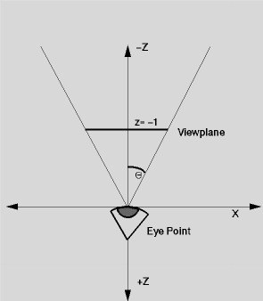
      In a simple ray caster you can trace the scene in a restricted world (eye) space by requiring the viewer to be at the origin, looking down the negative Z-axis


      To calculate the field of view, assume that your rays go from
      X: -tan(theta) to tan(theta)
      Y: -ratio*tan(theta) to ratio*tan(theta), where
      ratio = (Vyt - Vyb)/(Vxr - Vxl)

      General Algorithm Outline

         for each pixel 
       	Determine the closest object 
                along the ray from the eye pt. 
                through the pixel.
      	Find it's color.
              Set pixel color to this color.
      

      More Detailed Algorithm

      • Read in scene information and object information
      • Initialize color table (using ct_gen)
      • Calculate viewing parameters and area to raytrace
      • For Y = -ratio*tan(theta) to ratio*tan(theta)
        • Initialize color_buffer to background color
        • For X = -tan(theta) to tan(theta)
          • For each object in the scene
            • Test to see if ray intersects each object and save t value of this intersection and object number if this is the closest one so far.
          • Shoot shadow rays for this pixel for the closest object
          • Calculate the illumination and color of this object based on the illumination model.
          • color_buffer[x] = color from above
        • Write color_buffer to screen or file (using write_buffer cmd)

    2. Z-Buffer Algorithm:
      • We know how to scan-convert polygons onto the screen.

      • What we want to do now is, only overwrite a pixel if the polygon element has a larger Z value than what is in the frame-buffer currently.

      • We will create a Z-buffer to hold the depth values of each pixel in the frame-buffer.

      • The general Algorithm:
        	Initialize frame-buffer and Z-buffer
        
           	for each polygon P
        	  for each pixel in poly's projection:  x,y
        		pz = the Z value of P at this pixel
        		polycolor[x][y] = 
        			color of P at this pixel
        		if Z-buffer[x][y] <=  pz
        			Z-buffer[x][y] = pz
        			FB[x][y] = polycolor[x][y]
        	  end for each pixel
               end for each polygon
                  
      • Z values calculated incrementally from the plane equation (dz/dx, dz/dy).

      • Number of comparisons independent of number of polygons.

      • Works fine for patches & other primitives.

      • Requires a large amount of memory (1280*1024*32bits typically > 5Mb)

      • Often implemented in hardware.


    3. Scanline Z-buffer
      • Instead of storing an entire Z-buffer, what if we store only 1 scanline at a time to save memory ?

      • How does the algorithm have to change?

      • We switch the order of the for loops.
           Initialize scanline color-buffer CB and Z-buffer
        
           for each scanline
             for each polygon P active in the scanline
        	for each x in poly's projection
         	   pz = the Z value of P at this pixel
        	   polycolor[x][y] = color of P at this 
        		pixel
        	   if Z-buffer[x] <=  pz
        		Z-buffer[x] = pz
        		CB[x] = polycolor[x][y]
        	end for each x
             end for each polygon
             draw the  color-buffer CB to the screen
           end for each scanline
                

      • What are the disadvantages of this algorithm compared to the Z-buffer algorithm?


    4. Warnock's Algorithm:

      • Screen-Space Subdivision.

      • A polygon's relation to an area is one of 4 cases:

        See Figure 15.42 from F&vD pg 687.

        1. Completely surrounds it.
        2. Intersects it.
        3. Is contained in it.
        4. Disjoint (is outside the area)

      • If one of the four cases below doesn't hold, then subdivide until it does:

        1. All polys are disjoint wrt the area =>
          draw the background color

        2. 1 intersecting or contained polygon =>
          draw background, then draw contained portion of the polygon.

        3. There is a single surrounding polygon =>
          draw the area in the polygon's color.

        4. There is a front surrounding polygon =>
          draw the area in the polygon's color.

      • Recursion stops when you are at the pixel level, or lower for anti-aliasing.

      • At this point do a depth sort and take the polygon with the closest Z value.

      • Most of the work is done at the object space level.

      • An Example: See Figure 15.44 from F&VD p 688

    5. Spanning Scanline (Walkins, Romney)

      • fewer depth comparisons
      • uses spans -- divide scanline at each edge crossing => spans
      • 3 span cases
        • empty --> draw background
        • contain only 1 segment --> display on screen
        • contain only multiple segments --> calculate depth of each span draw one with smallest z
          • if penetration allowed, divide span at point of intersection.
      • simple modification of scanline Z-buffer.
      • need to check for intersecting edge in a span (sign of end point difference change).


      Return to CMSC 635 Notes Page


      Last modified: Mon Feb 15 14:24:40 EST 1999