<- previous index next ->
Digital Filtering uses numerical computation rather than analog
components such as resistors, capacitors and inductors to
filter out frequency bands.
A low-pass filter will have a "cutoff frequency" f such that
frequencies above f will be attenuated and frequencies below f
will be passed. The filter does not produce a sharp dividing
line and all frequencies are changed in both amplitude and
phase angle.
A high-pass filter will have a "cutoff frequency" f such that
frequencies below f will be attenuated and frequencies above f
will be passed. The filter does not produce a sharp dividing
line and all frequencies are changed in both amplitude and
phase angle.
A band-pass filter will pass frequencies between f1 and f2,
attenuating frequencies below f1 and attenuating frequencies
above f2. f1 <= f2.
The signal v(t)=sin(2 Pi f t) t=t0, t1, ..tn is a single frequency f.
For digital filtering we assume the digital value of v(ti) is
sampled at uniformly spaced times t0, t1,..., tn.
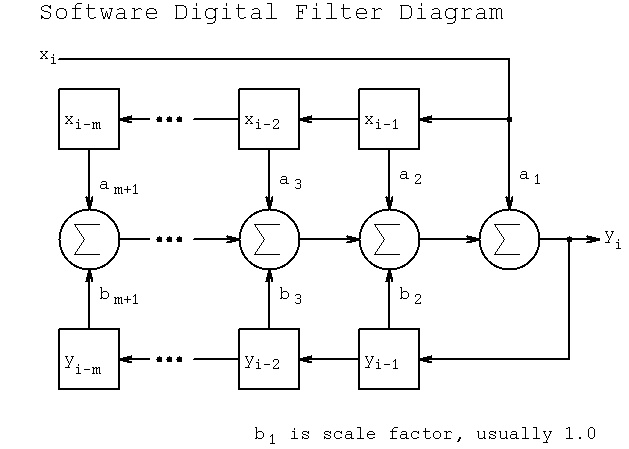
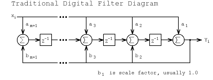 For an order m filter, with one based subscripts:
y(i) = ( a(1)*x(i) + a(2)*x(i-1) + a(3)*x(i-2) + ... + a(m+1)*x(i-m)
- b(2)*y(i-1) - b(3)*y(i-2) - ... - b(m+1)*y(i-m) )/b(1)
For an order m filter, with one based subscripts:
y(i) = ( a(1)*x(i) + a(2)*x(i-1) + a(3)*x(i-2) + ... + a(m+1)*x(i-m)
- b(2)*y(i-1) - b(3)*y(i-2) - ... - b(m+1)*y(i-m) )/b(1)
 With array x and y in memory, the MatLab code for computing y(1:n) could be:
for i=1:n
y(i)=a(1)*x(i);
for j=1:m
if j>=i
break
end
y(i)=y(i) + a(j+1)*x(i-j) - b(j+1)*y(i-j);
end
y(i)=y(i)/b(1); % not needed if b(1) equals 1.0
end
or, use MatLab y = filter(a, b, x); % less typing
For an order m filter, with zero based subscripts:
y[i] = ( a[0]*x(i) + a[1]*x[i-1] + a[2]*x[i-2] + ... + a[m]*x[i-m]
- b[1]*y[i-1] - b[2]*y[i-2] + ... - b[m]*y[i-m] )/b[0]
With array x and y in memory, the C code for computing y[0] to y[n-1] could be:
for(i=0; i<n; i++) {
y[i]=a[0]*x[i];
for(j=1; j<=m; j++)
{
if(j>i) break;
y[i]=y[i] + a[j]*x[i-j] - b[j]*y[i-j];
}
y[i]=y[i]/b[0]; /* not needed if b[0]==1 */
}
For reading x samples and writing filtered y values:
read next x sample and compute y and output y
(the oldest x and y in RAM are deleted and the new x and y saved.
Typically use a circular buffer [ring buffer] so that the saved x and y
values do not have to be moved [many uses of modulo in this code].)
Given a periodic input, filters require a number of samples to build up
to a steady state value. There will be amplitude change and phase change.
Typical symbol definitions related to digital filters include:
ω = 2 Π f
z = ej ω t digital frequency
s = j ω analog frequency
z-1 is a unit delay (previous sample)
IIR Infinite Impulse Response filter or just recursive filter.
In transfer function form
yi a0 + a1 z-1 + a2 z-2 + a3 z-3 + ...
---- = -----------------------------------
xi b1 z-1 + b2 z-2 + b3 z-3 + ...
s = c (1-z-1)/(1+z-1) bilinear transform
db = 10 log10 (Power_out/Power_in) decibel for power
db = 20 log10 (Voltage_out/Voltage_in) decibel for amplitude
(note that db is based on a ratio, thus amplitude ratio may
be either voltage or current. Power may be voltage squared,
current squared or voltage times current. More on db at end.)
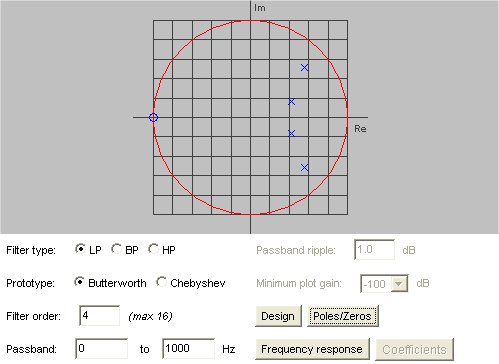
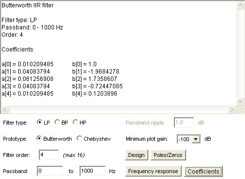
A Java program is shown that computes the a and b coefficients for
Butterworth and Chebyshev digital filters. Options include Low-Pass,
Band-Pass and High-Pass for order 1 through 16. Click on the sequence:
Design, Poles/Zeros, Frequency response, coefficients to get output
similar to the screen shots shown below.
The Pole/Zero plot shows the complex z-plane with a unit circle.
The poles, x, and zeros o may be multiple.
With array x and y in memory, the MatLab code for computing y(1:n) could be:
for i=1:n
y(i)=a(1)*x(i);
for j=1:m
if j>=i
break
end
y(i)=y(i) + a(j+1)*x(i-j) - b(j+1)*y(i-j);
end
y(i)=y(i)/b(1); % not needed if b(1) equals 1.0
end
or, use MatLab y = filter(a, b, x); % less typing
For an order m filter, with zero based subscripts:
y[i] = ( a[0]*x(i) + a[1]*x[i-1] + a[2]*x[i-2] + ... + a[m]*x[i-m]
- b[1]*y[i-1] - b[2]*y[i-2] + ... - b[m]*y[i-m] )/b[0]
With array x and y in memory, the C code for computing y[0] to y[n-1] could be:
for(i=0; i<n; i++) {
y[i]=a[0]*x[i];
for(j=1; j<=m; j++)
{
if(j>i) break;
y[i]=y[i] + a[j]*x[i-j] - b[j]*y[i-j];
}
y[i]=y[i]/b[0]; /* not needed if b[0]==1 */
}
For reading x samples and writing filtered y values:
read next x sample and compute y and output y
(the oldest x and y in RAM are deleted and the new x and y saved.
Typically use a circular buffer [ring buffer] so that the saved x and y
values do not have to be moved [many uses of modulo in this code].)
Given a periodic input, filters require a number of samples to build up
to a steady state value. There will be amplitude change and phase change.
Typical symbol definitions related to digital filters include:
ω = 2 Π f
z = ej ω t digital frequency
s = j ω analog frequency
z-1 is a unit delay (previous sample)
IIR Infinite Impulse Response filter or just recursive filter.
In transfer function form
yi a0 + a1 z-1 + a2 z-2 + a3 z-3 + ...
---- = -----------------------------------
xi b1 z-1 + b2 z-2 + b3 z-3 + ...
s = c (1-z-1)/(1+z-1) bilinear transform
db = 10 log10 (Power_out/Power_in) decibel for power
db = 20 log10 (Voltage_out/Voltage_in) decibel for amplitude
(note that db is based on a ratio, thus amplitude ratio may
be either voltage or current. Power may be voltage squared,
current squared or voltage times current. More on db at end.)
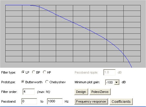
A Java program is shown that computes the a and b coefficients for
Butterworth and Chebyshev digital filters. Options include Low-Pass,
Band-Pass and High-Pass for order 1 through 16. Click on the sequence:
Design, Poles/Zeros, Frequency response, coefficients to get output
similar to the screen shots shown below.
The Pole/Zero plot shows the complex z-plane with a unit circle.
The poles, x, and zeros o may be multiple.
 The frequency response is for the range 0 to 4000 Hz based on
the 8000 Hz sampling. 0 db is at the top, the bottom is the
user selected range, -100 db is the default.
The frequency response is for the range 0 to 4000 Hz based on
the 8000 Hz sampling. 0 db is at the top, the bottom is the
user selected range, -100 db is the default.
 The coefficients are given with zero based subscripts.
(These subscripts may be used directly in C, C++, Java, etc.
add one to the subscript for Fortran, MatLab and diagrams above.)
The coefficients are given with zero based subscripts.
(These subscripts may be used directly in C, C++, Java, etc.
add one to the subscript for Fortran, MatLab and diagrams above.)
 Note that MatLab has 'wavread' and 'wavwrite' functions as well
as a 'sound' function to play .wav files. 'wavwrite' writes
samples at 8000 Hz using the default.
The files to compile and run the Digital Filter coefficients are:
IIRFilterDesign.java
IIRFilter.java
PoleZeroPlot.java
GraphPlot.java
make_filter.bat
Makefile_filter
mydesign.out
This is enough for you to be able to program and use simple
digital filters. This lecture just scratched the surface.
There are many types of digital filters with many variations.
There are complete textbooks on just the subject of digital filters.
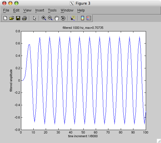
The output from the low pass filter shown above "builds up and settles"
quickly:
Note that MatLab has 'wavread' and 'wavwrite' functions as well
as a 'sound' function to play .wav files. 'wavwrite' writes
samples at 8000 Hz using the default.
The files to compile and run the Digital Filter coefficients are:
IIRFilterDesign.java
IIRFilter.java
PoleZeroPlot.java
GraphPlot.java
make_filter.bat
Makefile_filter
mydesign.out
This is enough for you to be able to program and use simple
digital filters. This lecture just scratched the surface.
There are many types of digital filters with many variations.
There are complete textbooks on just the subject of digital filters.
The output from the low pass filter shown above "builds up and settles"
quickly:
 A fourth order band pass filter with band 2000 to 2100 requires
more samples for the center frequency 2050 to build up and settle:
A fourth order band pass filter with band 2000 to 2100 requires
more samples for the center frequency 2050 to build up and settle:
 Some notes on db
+3 db is twice the power
-3 db is half the power
+10 db is ten times the power
-10 db is one tenth the power
+30 db is 1000 times the power, 10^3
-30 db is 1/1000 of the power, 10^-3
+60 db is one million times the power, 10^6
-60 db is very small
Sound is measured to average human hearing threshold,
technically 20 micropascals of pressure by definition 0 db.
Some approximate examples for sound from a close source:
0 db threshold of hearing
20 db whisper
60 db normal conversation
80 db vacuum cleaner
90 db lawn mover
110 db front row at rock concert
130 db threshold of pain
140 db military jet takeoff, gun shot, fire cracker
180 db damage to structures
194 db shock waves begin, not normal sound
The sound drops off with distance by the inverse square law.
Each time you move twice as far away from the source,
the sound is 1/4 as strong.
The effective loudness decreases with very short burst of sound.
160 db for 1/100 second is about a loud as 140 db for 1 second.
Sample db vs power code
dbtopower.c source
dbtopower_c.out results
dbtopower.py source
dbtopower_py.out results
Some notes on db
+3 db is twice the power
-3 db is half the power
+10 db is ten times the power
-10 db is one tenth the power
+30 db is 1000 times the power, 10^3
-30 db is 1/1000 of the power, 10^-3
+60 db is one million times the power, 10^6
-60 db is very small
Sound is measured to average human hearing threshold,
technically 20 micropascals of pressure by definition 0 db.
Some approximate examples for sound from a close source:
0 db threshold of hearing
20 db whisper
60 db normal conversation
80 db vacuum cleaner
90 db lawn mover
110 db front row at rock concert
130 db threshold of pain
140 db military jet takeoff, gun shot, fire cracker
180 db damage to structures
194 db shock waves begin, not normal sound
The sound drops off with distance by the inverse square law.
Each time you move twice as far away from the source,
the sound is 1/4 as strong.
The effective loudness decreases with very short burst of sound.
160 db for 1/100 second is about a loud as 140 db for 1 second.
Sample db vs power code
dbtopower.c source
dbtopower_c.out results
dbtopower.py source
dbtopower_py.out results
<- previous index next ->
-
CMSC 455 home page
-
Syllabus - class dates and subjects, homework dates, reading assignments
-
Homework assignments - the details
-
Projects -
-
Partial Lecture Notes, one per WEB page
-
Partial Lecture Notes, one big page for printing
-
Downloadable samples, source and executables
-
Some brief notes on Matlab
-
Some brief notes on Python
-
Some brief notes on Fortran 95
-
Some brief notes on Ada 95
-
An Ada math library (gnatmath95)
-
Finite difference approximations for derivatives
-
MATLAB examples, some ODE, some PDE
-
parallel threads examples
-
Reference pages on Taylor series, identities,
coordinate systems, differential operators
-
selected news related to numerical computation