Figure 1. Simplified view of the PixelFlow system
In the previous sections of this chapter, we covered the interface seen by both application and shader writers. In this section, we cover the basic knowledge of the PixelFlow hardware required to understand the implementation issues. For more details on the PixelFlow architecture, see [Molnar91][Molnar92][Eyles97]. We also cover some intermediate levels of abstraction between PixelFlow and an abstract graphics pipeline and explain how our procedural stages fit into the real PixelFlow pipeline.
Our abstract pipeline consists of procedures for each stage in the rendering process. Since these can be programmed completely independently, it is possible (and expected) that a particular hardware implementation may not have procedural interfaces for all stages. While PixelFlow is theoretically capable of programmability at every stage of the abstract pipeline, our implementation only provided high-level language support for surface shading, lighting, and primitives. The underlying PixelFlow software includes provisions for programmable testbed-style atmospheric and image warping functions, but we did not supply any special-purpose language support for these.
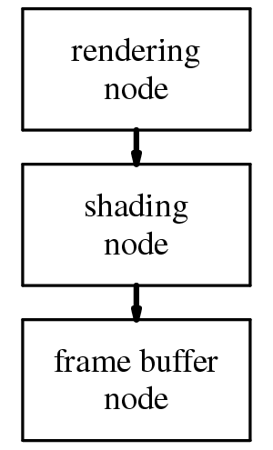
The modeling, transformation, primitive, and interpolation stages are handled by the rendering node. The shading, lighting, and atmospheric stages are handled by the shading node. Finally, the image warping stage is handled by the frame buffer node.
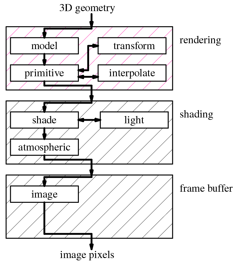
It is important to notice that the abstract pipeline only provides a conceptual view for programming the stages. It allows the procedure programmer to pretend that the machine is just a simple pipeline instead of a large multicomputer. The real stages do not need to be executed strictly in the order given (and, in fact, are not). The user writing code for one of the stages does not need to know the differences between the execution order given in the abstract pipeline and the true execution order. The mapping of the abstract pipeline onto PixelFlow exhibits several different forms of this.
The first example is the overall organization of the processes on PixelFlow. PixelFlow completes all of the modeling, transformation, primitives, and interpolation in the rendering nodes before sending the shading parameters for the visible pixels on to a shading node. PixelFlow then completes all of the shading, lighting, and atmospheric effects before sending the completed pixels on to the frame buffer node for warping. On a different graphics architecture, it might make more sense to complete all of the stages for every pixel in a primitive before moving on to the next primitive. Either choice appears the same to users who write the procedures. The abstract pipeline does not include information about the stage scheduling to allow just such implementation flexibility.
The procedures running on the PixelFlow rendering nodes provide another example. The abstract pipeline presents transformation, primitive, and interpolation as if they were a sequential chain of processes. On PixelFlow, the primitive stage drives transformation and interpolation. A procedural primitive function is invoked for each primitive to be rendered. This function calls both transformation and interpolation functions on demand as needed. The results stored for each pixel include its depth, an identifier for which procedural shader to use and the shading parameters for that procedural shader. Once again, the user writes procedures as if they were independent sequential stages and is not aware of the true ordering within the PixelFlow implementation.
The final example is with the shading and lighting stages. The abstract pipeline presents shading and lighting as if the shading stage called the lighting stage for each light. On PixelFlow, the linkage between these stages is not as direct. These two stages run with an interleaved execution scheduled by the PixelFlow software system. This interleaving is explained in more detail in [Olano98]. And again, the interleaved scheduling is hidden from anyone who writes a shading or lighting procedure.
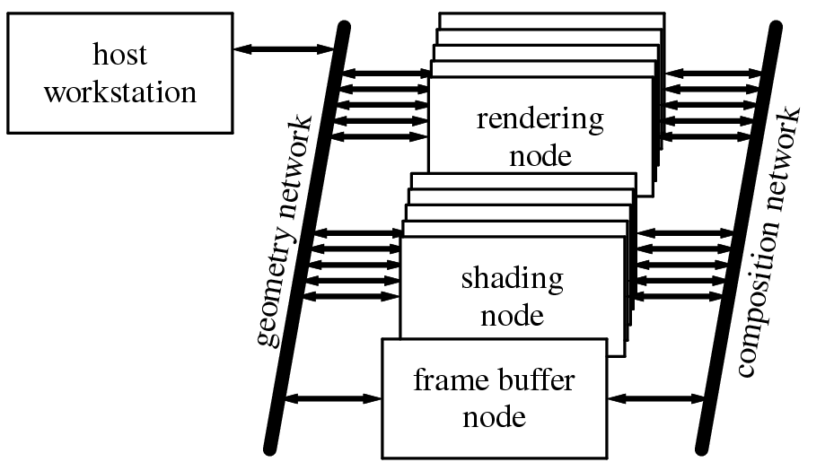
Since each rendering node has only a subset of the primitives, a region rendered by one node will have holes and missing polygons. The different versions of the region are merged using image composition. PixelFlow includes a special high-bandwidth network called the composition network with hardware support for these comparisons. As all of the rendering nodes simultaneously transmit their data for a region, the network hardware on each node compares, pixel-by-pixel, the data it is transmitting with the data coming in from the upstream nodes. It keeps only the closest of each pair of pixels to send downstream. By the time all of the pixels reach their destination, one of the shading nodes, the composition is complete.
Once a shading node has received the data, it does the surface shading for the entire region. The technique of shading after the pixel visibility has been determined is called deferred shading [Deering88][Ellsworth91]. Deferred shading only spends time shading the pixels that are actually visible, and allows us to do shading computations for many more pixels in parallel. With non-deferred shading, each primitive is shaded separately. With deferred shading, all primitives in a region that use the same procedural shader can be shaded at the same time.
In a PixelFlow system with n shading nodes, each
shades every nth region. Once each region has
been shaded, it is sent over the composition network (without
compositing) to the frame buffer node, where the regions are collected
and displayed.
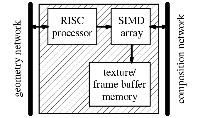
The compiler for our special-purpose language produces C++ code that exactly conforms to the testbed interface. This code consists of two functions, a load function (mentioned in section 1.2), and the actual code for the procedure. The code for the procedure is run on the RISC processor and includes embedded EMC functions. Each EMC function puts one SIMD instruction into an instruction stream buffer. The EMC prefix that appears on all of these functions stands for enhanced memory controller, from the Pixel-Planes SIMD array's origin as a processor-enhanced memory; we use it here just to identify the functions that generate the SIMD instruction stream.
When the C++ code for a procedure is run, the result is a buffer full of instructions for the SIMD array. This instruction stream buffer can be sent to the SIMD array several times without requiring the original C++ code to be re-executed.
There are two forms of EMC function used in PixelFlow. The form used on the shading nodes checks the available space in the instruction stream buffer with each instruction and can re-allocate the buffer on the fly. The form used in the rendering nodes requires a buffer of sufficient size to be allocated at the beginning of the procedure. The reason for this difference, and the issues that result, are discussed in Section [Olano99].