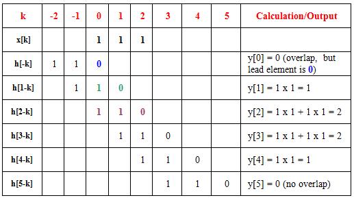
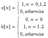
We now explain the steps in the above table. Firstly x[n] = [1 1 1] and h[n] = [0 1 1] (see the definitions), but we have taken h[n] and “flipped” it or made a mirror image of it, h[-n] = [1 1 0]. We have also moved this new array as far left as we can take it so that it just overlaps x[k] (see table, 3^rd row). In this position the two numbers that overlap in the column that has 0 at the top is 1 and 0. The product 1 x 0 = 0 and that is the output. Now take the row h[1-k] where the overlap is in the 0^th and 1^st columns. The product is 1 x 1 + 1 x 0 = 1. Note how h[1-k] is essentially the same as h[-k], but is slid over to the right by one position. Similarly, consider h[2-k]. Now the overlap is in the 0^th, 1^st and 2^nd columns. The product is 1 x 1 + 1 x 1 + 1 x 0 = 2. The student should now be able to do the rest of the calculation. Note how h[k] had 3 elements [0 1 1] and x[k] also had 3 elements [1 1 1]. However, the output y[n] has 5 elements [0 1 2 2 1]. In general if x[n] has N elements and h[n] has K elements, then y[k] will have N+K-1 elements.

Method 2

It is important to note again (as seen in the last sentence of the previous paragraph) that x[n] and h[n] need not be the same length. As it turns out, h[n] can be fairly short in length whereas, x[n] is not restricted to be so. In fact, in the signal processing literature, h[n] is called the filter and x[n] the signal. Now if the signal is say a performance of the pop song “Seven Nation Army” by the White Stripes, then the signal is going to be a vector of a few million elements while the filter h[n] may be less than 100 elements long. Loading the entire signal x[n] into memory is not a very sensible option. Luckily mathematics comes to the rescue. The convolution operation as defined by EQUATION (1) remains the same, but some additional steps are necessary. Here is how you should proceed. Consider x = [1,1,2,1,2,2,1,1] (comma separated) and break it into three contiguous sub-blocks x0 = [1,1,2], x1 = [1,2,2] and x2 = [1,1,0]. Note, we have added a 0 to x2 in order to make it have a length of three. The vector and sub-blocking process is shown below.

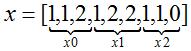
Note that x0 starts at position 0 in the original vector x. Similarly x1 starts at position 3 in vector x and x2 starts at position 6 in vector x – assuming indexing begins at 0. We will use this fact below.

Now consider a vector h = [1, 2, -1, 1]. Since both x and h have small lengths, we can do direct convolution as explained in method 1 – I leave that as an exercise for the students. Let us instead use a method that allows efficient use of memory. Form the three sub-convolutions (now each of h, x0, x1, and x2 are nearly the same length).

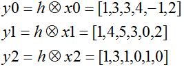
Now align the outputs y0, y1 and y2 as shown in the table below.

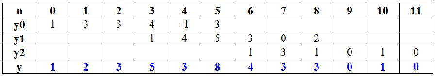
So the output is given by the particular alignment of y0 at position 0, y1 and position 3 and y2 at position 6 (mentioned earlier) and addition. There are 8 elements in the original x vector and 4 elements in h, therefore the convolution will produce 8+4-1=11 elements as output. If you look at the table above, there are 12 columns (with the 11^th column being redundant and inserted for completeness sake). How about the memory requirements for method 1 versus method 2? Method 1 requires x, h and the output y to be in memory or 8 + 4 + 11 = 23 elements. In method 2 you will read in x in blocks of 3 elements, h has 4 elements and any of y0, y1 and y2 will have 4 + 3 -1 = 6 elements. Also, we have to account for the overlapped elements of y0, y1 and y2. The overlapped elements will be 6 (length of convolution output of h and x0) – 3 (length of y0) = 3 elements. So at any time you will have 3 + 4 + 6 +3 = 16 elements in memory. Compare 23 elements for method 1 for 16 elements for method 2. While this may not seem like much, if N, the size of x grows large, the memory savings can be quite large.

So in general we break x into blocks of L (you may have to pad the last block with 0s to make it of length L). Each block is convolved with a filter h of length M. For this scheme to work L > M. The output of each block convolution is L+M-1 elements. If we start indexing with 0 then the next block convolution will start at L, the next block will start at 2L etc.

Here is pseudo code to do the convolution (blockcon)

Input h (length M) and block x (length L) (the filter and the data block)

1. Compute output (using method 1 or other method)

2. for i = 0,1, …, M-1
         y(i) = y(i) + y_temp(i) (overlap)
         y_temp(i) = y(i+L) (save tail)

The algorithm above uses an M dimensional vector y_temp to store the appropriate samples of the block. For the first block, y_temp needs to be initialized to 0. The student should follow the algorithm and see if it matches the output of the above table.

Here is pseudo code as to how your algorithm may work :

for () {Keep reading input blocks except last block which is treated separately
           blockcon()
           process input block that was just read input length of x is L and h is M
           write output block created by blockcon() to file
}
blockcon()                                                               Last block will an x that has number of elements N <= L. h remains length M
Write output block created by blockcon(S) to file

References:
The following books are suggested reading if you want to get into the nitty-gritty of signal processing.
Oppenheim, A. V., Shafer, R. W. and Buck, J. R., Discrete-Time Signal Processing, 2^nd ed., Prentice Hall, 1999
Proakis, J. G. and Manolakis, J. G. , Digital Signal Processing, 4^th ed, Prentice Hall, 2007
Mandal, M.and Asif, A. , Continuous and Discrete Time Signals and Systems, Cambridge University Press, 2007

Part 1: Add the system calls to the kernel.

• long setAWK421(const char *buf, unsigned long size); - Retrieve data in the userspace address provided by buf and store size bytes in kernelspace for later processing and retrieval. Returns the number of bytes successfully copied or a negative number to indicate a failure.
• long getAWK421(char *buf, unsigned long size); - Retrieve the processed data stored in kernelspace and store size bytes in the userspace address provided by buf. Returns the number of bytes successfully copied or a negative number to indicate failure. This syscall will fail if no active filter exists.
• long addAWKFilter421(const char *filter, unsigned long size); - Adds a new convolution filter to the kernel. Returns a filter ID number or a negative number to indicate a failure.
• long setAWKFilter421(long id); - Sets the filter id as the active filter, which is the filter used when data is retrieved. Returns the id if successful, 0 indicating the filter id does not exist, or a negative number to indicate any other failure.
• long delAWKFilter421(long id); - Remove the filter identified by id from the list of available filters. Returns the id if successful, 0 indicating the filter id does not exist, or a negative number to indicate any other failure. If the filter is the active filter, set another available filter as the active filter, or indicate that there are no active filters.
• long listAWKFilterID421(long *fids, unsigned long size); - Store a list of up to size filter id numbers starting at the userspace address indicated by fids. Return the number of filters stored or a negative number to indicate a failure.
• long clearAWK421(); - Resets the buffer (note that this leaves the filters alone). Should return 0, unless there is a catastrophic failure/data corruption that prevents the data from being cleared.

You may assume that there are at most 256 possible filters. Each of which are at most 512 bytes long. You may also assume that the largest data buffer you can store is 1K, or 1024 bytes. Do not assume that the filters are null terminated strings or that they or their results are printable characters.

Make sure that your system calls have exactly the same signatures as above, otherwise our test programs will fail and thus your assignment as well. Your underlying implementation is your decision. You will need to explain the pros and cons of your decisions in your report file.

N.B. System calls can be called concurrently, you will need to lock your internal structures to make sure that access to them is mutually exclusive (otherwise two processes writing to your data at the same time will produce very interesting results).

N.B. We never specified when the data was processed in the description above. You should pick and explain why you chose that option in your report.

Part 2: User mode driver and test programs

Now that you have system calls created to provide the interface, your PHB demands that you write a reference implementation to show the other programmers how to use it. He wants three programs:

1. loadfilters <file> - Takes a file with a list of filter file names and loads each filter into the kernel. The file should be given as the only command line parameter. This program should print a list of filter ids back to the command prompt.
2. fcm - The "Filter Commander" provide an interactive interface to the user to provide the following functions:
   • List, Select, Add, Remove filters. Should ask for a filename or id number as required.
   • Clear, Save, or Load messages. Should ask for a filename and the amount of data to be processed for each operation.
3. proclarge <infile> <outfile> <fid> - Process a large infile and store it in outfile using the filer identified by fid. The fid command is optional, and even if the id given does not exist the system should use the active filter. This command should clear any previously existing buffer data.

Filter and message files are raw data files, not ascii. Each program should detect and report any errors thrown by the system on stderr, and any other useful information (e.g. the number of bytes successfully processed or sent) should be reported to stdout.

N.B. You should use your own test program to test your system calls to ensure that they work as specified and they can handle all kinds of (good and bad) inputs. Include these extra programs in your submission.

Part 3: Project Questions

• How does errno work?
• What synchronization method did you use? What other kernel synchronization methods are available, and how would you use them? Which method is the best for the given problem? Which is the worst? Why did you choose the one you chose?
• What other ways could you have chosen to store the data you needed to store in the kernel? Discuss the pros and cons of each relative to what you chose.
• The project description states that a loadable module or driver compiled into the kernel would be better, why?
• How do system calls work? Explain the entire execution path from userspace to kernelspace and back, and be specific to the intel ia32/x86 architecture.

Hints & References

• Creating A Simple System Call in the 2.6 Linux Kernel
• A tutorial on adding a System Call from WPI
• Kernel Korner: System Calls
• Linux Resources
• Recall that a system call is a software trap or interrupt. This means that when adding a new system call, you will need to update the system call dispatch table (i.e. the interrupt vector) with new entry/entries, and generate stub(s) that will be used by user programs.
• You should always check the validity of addreeses in the user address space passed to your system calls, and use appropriate functions from the Kernel API whenever transfering data between kernel and user address space (see User Space Memory Access, the Kernel API, and related links in the Class Linux Resources).
• In the critical section of the code you write (e.g. when you access the new kernel variables), you should try to avoid any race conditions by using appropriate kernel locking. Refer to LKD for examples and discussion.

What to submit

Your patchfile should be named patchprj1.diff. Many students have made the mistake of misnaming their patch or putting it in the wrong directory in project 0. It should be located in the base directory. You should test your patch to make sure that it works. If it does not work or is in the wrong directory, it can have a significant impact on your grade. If you do nothing else, be absolutely 100% sure that your patch is working, named correctly, and in the right location in your submission archive!

Use the guidelines provided by project 0. Everything from project 0 (config, readme, report, etc) is required for all projects. Be sure to include any source files in the kernel that you changed or added to the kernel codebase (there should be several). Describe the organization of these files (where they were from relative to kernel sources v. where they are now) in your readme.

You should also be sure to include sample output showing the execution of your driver programs (this can be obtained by running the "script" command and submitting the file "typescript" generated as output by script). Students often forget this step.

It is very important for your grade that your project submission be well organized and that you make it very clear what you have done. Grading each submission takes a significant amount of effort and time. The TAs will not waste their time searching your submission to find the required pieces, you will simply lose points if they can't find what they are looking for. While you may be able to get back some credit by meeting with a TA, this will waste both your and the TA's time. With this in mind, you should be ready to spend about 1-2hrs preparing and verifying your archive for submission.